This document briefly introduces ongoing work to enhance the 3D radiative transfer solver which is coupled to the DALES model. It turns out that strong aspect ratios lead to an enhanced downward direction of radiation propagation in the Tenstream radiative transfer solver. To overcome this, at least partially, I played with some implementations of higher order solvers.
We have now the following setup of solvers:
- 3_* — 3 for direct radiation (fixed angle, one on each face)
- 8_* — 8 for direct radiation (fixed angle, but higher order in the spatial discretization, i.e. 4 on top faces, 2 on sides)
- *_10 — 10 diffuse streams (on top faces, one up, one down and on sidefaces one stream going left down, one going right down and 2 upwards respectively
- *_16 — 16 diffuse streams (side streams staying the same but on top we have 4 streams going downwards/upwards, i.e. not azimuthally averaged anymore but we now have them seperate for each quadrant of azimuth
- *_18 — same as 16 but additionally one stream that captures all vertically straight radiation, i.e. azimuthally averaged with zenith angle between 0 and 70deg
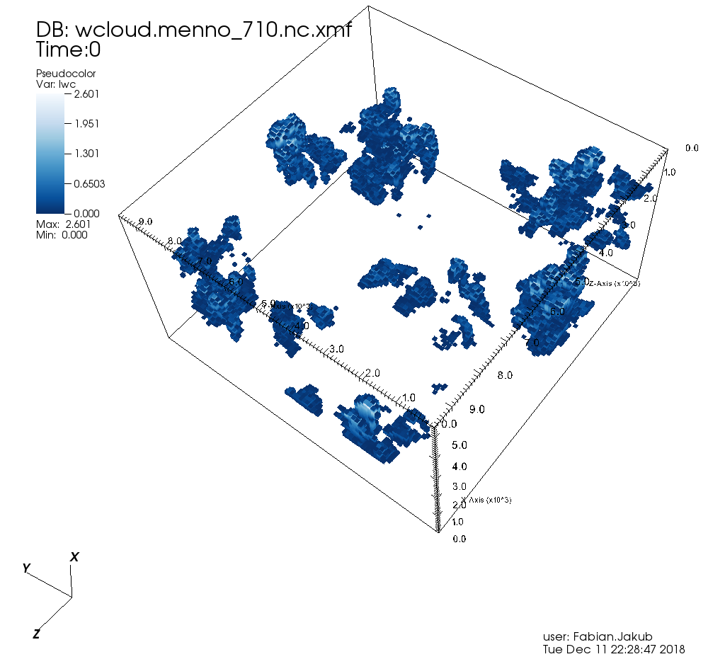
Comparison on the Cumulus cloud fields of Menno
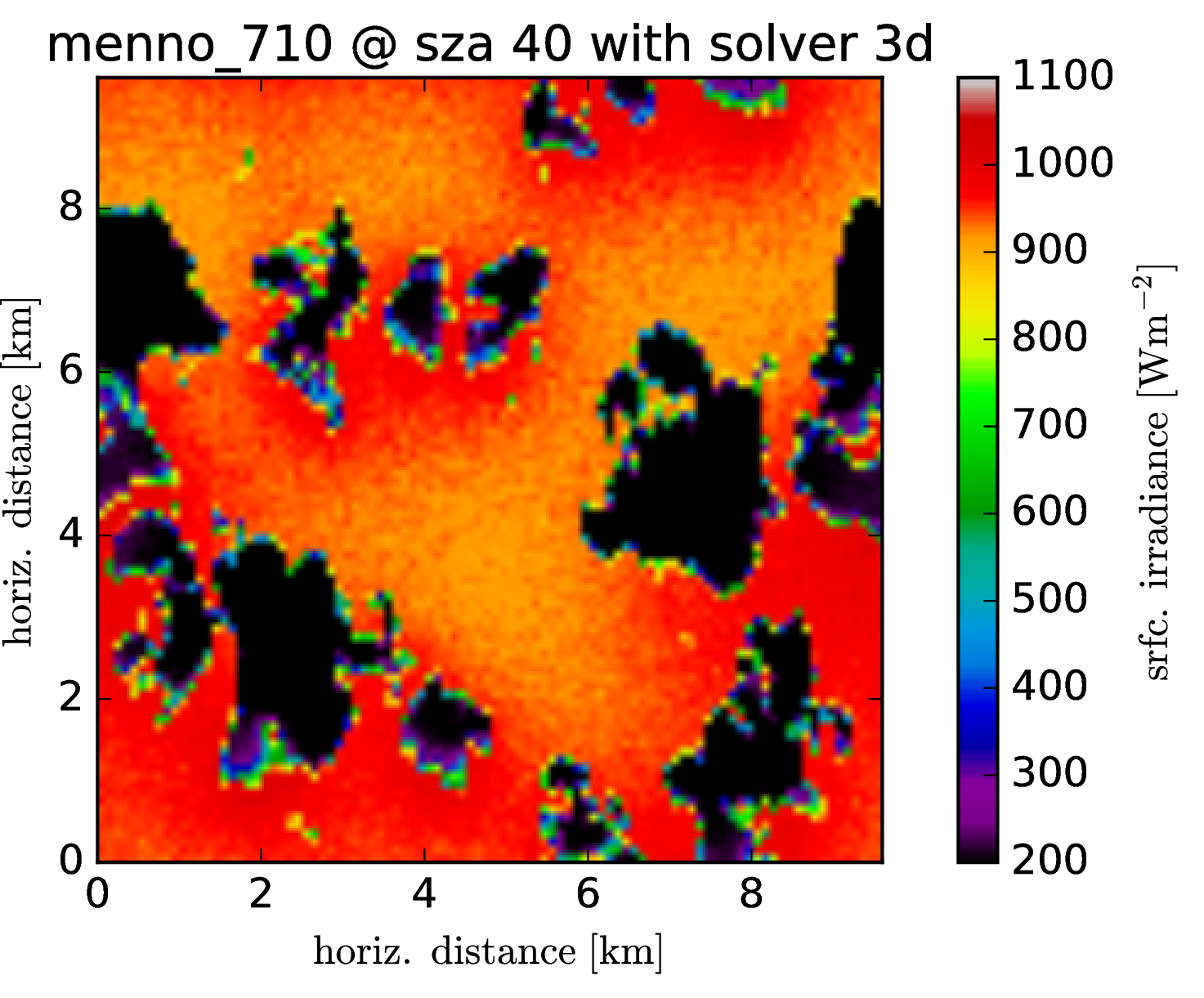
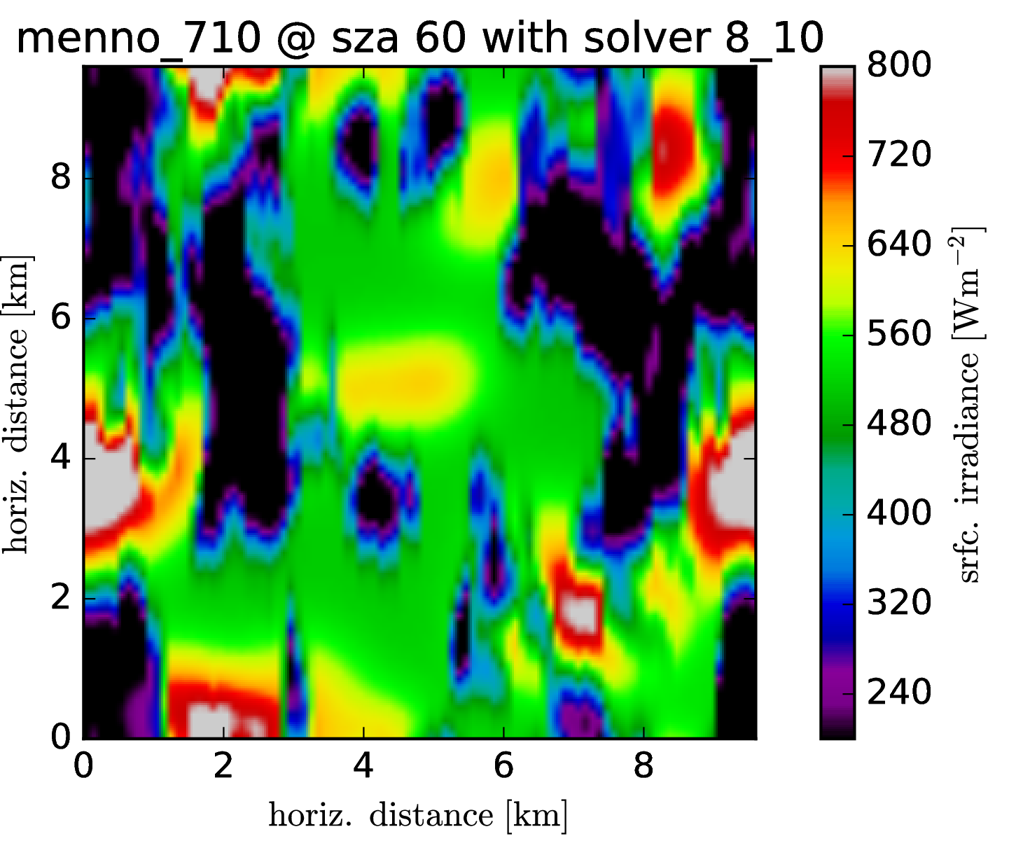
The cloud field has strong aspect ratios with horizontal resolution of 100m and a vertical resolution of 12m, encompassing 96 * 96 * 456 voxels. One particular problem, it seems, are the heat spots which are generated at the surface. It was known before that the Tenstream is not very diffusive with only two streams in the vertical and to represent the horizontal spread of diffuse radiation correctly, we now introduce 8 streams also for the vertical propagation of radiation.
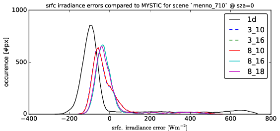
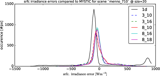
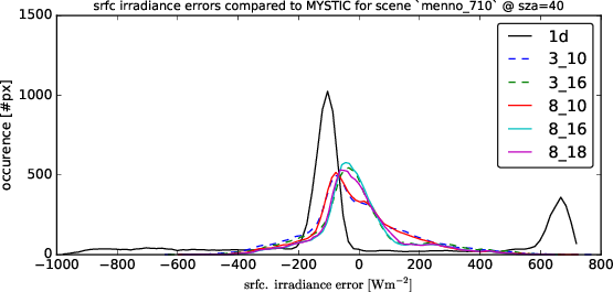
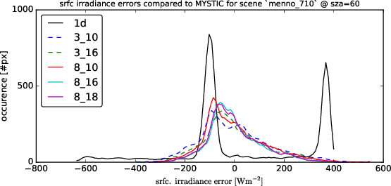
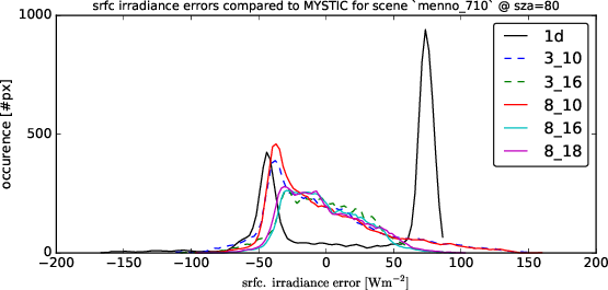
Following graphs show the error distributions for the total radiative flux at the surface for each solver compared to MonteCarlo benchmark simulations. I.e. histogram( E_srfc(*) - E_srfc(3D MYSTIC) ) for several solar zenith angles
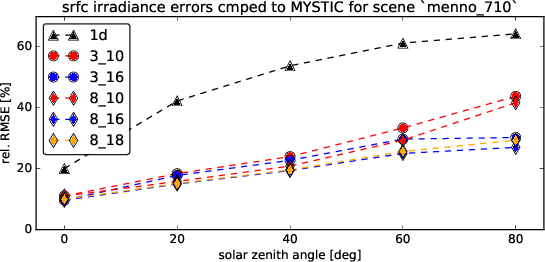
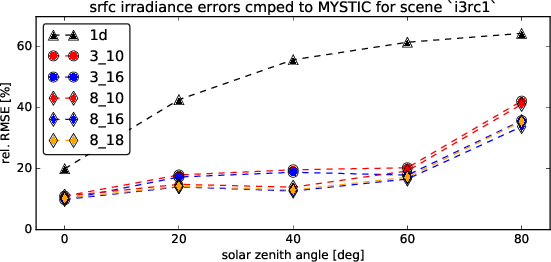
Following graph gives the relative Root Mean Squared Error for the individual solvers at several solar zenith angles.
Max difference [W/m2]
The following table gives the maximum difference between 1D and 3D surface fluxes:
max(abs(E_surface(*) - E_surface(MYSTIC)))
(sidenote: to account for montecarlo noise, I smoothed the difference fields with a 2D uniform filter with size 4)
| SZA [\(\ ^{\circ}\)] | 1D max. difference [W/m2] |
8_10 str max. difference [W/m2] |
8_16 str max. difference [W/m2] |
|---|---|---|---|
| 0 | 356 | 195 | 136 |
| 20 | 905 | 210 | 157 |
| 40 | 898 | 295 | 186 |
| 60 | 602 | 271 | 132 |
| 80 | 92 | 123 | 44 |
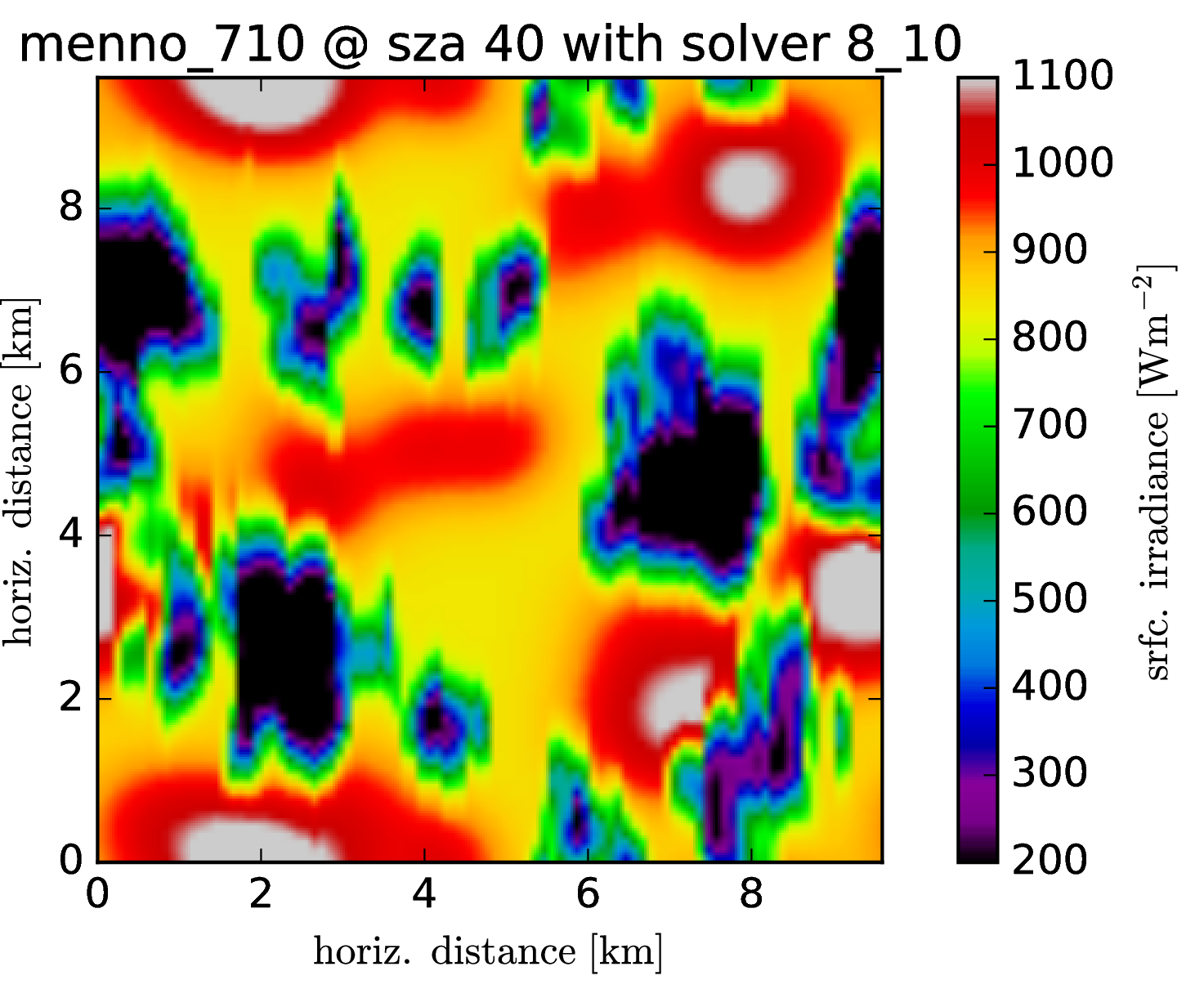
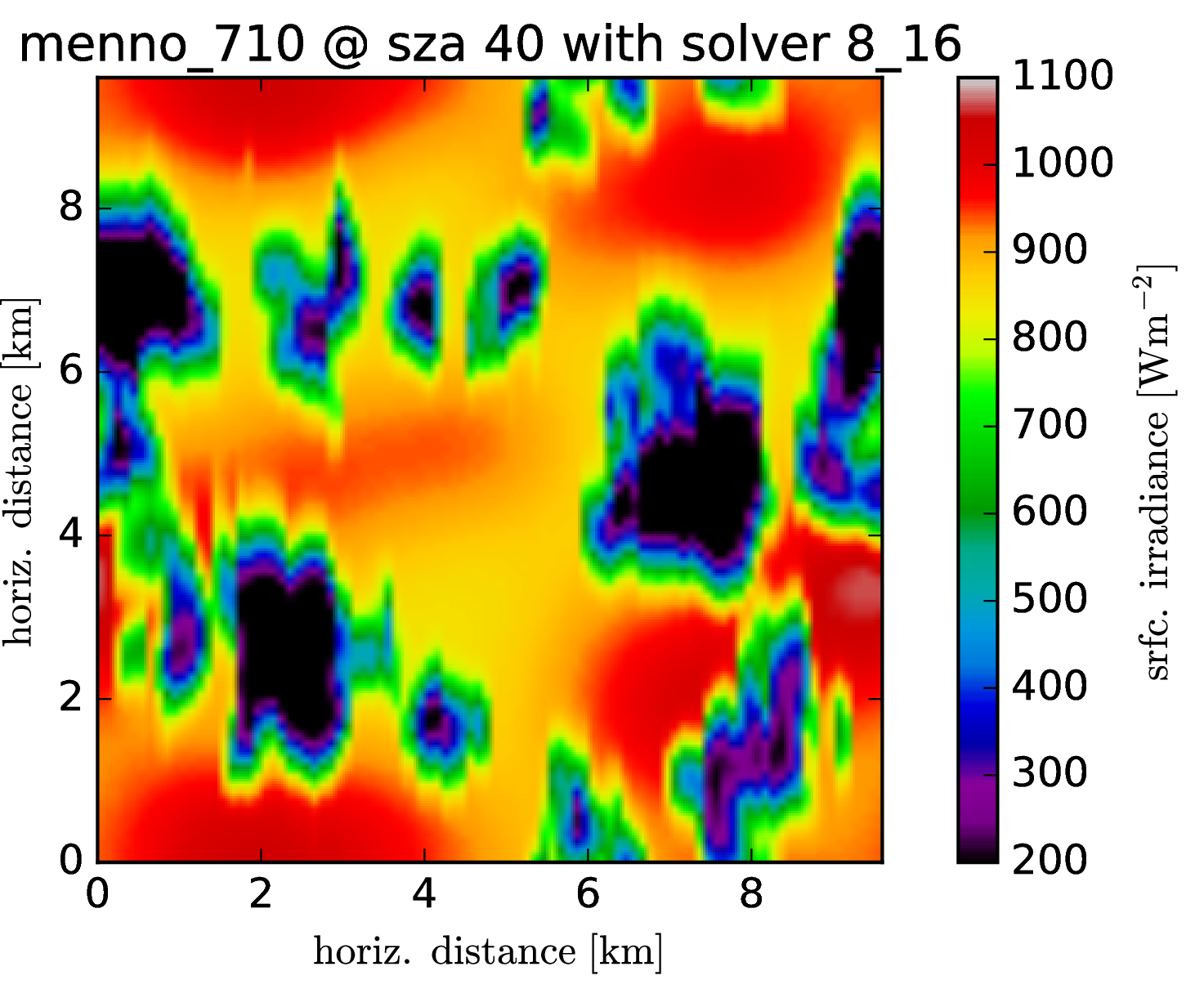
Srfc irradiance (direct + diffuse) SZA 40

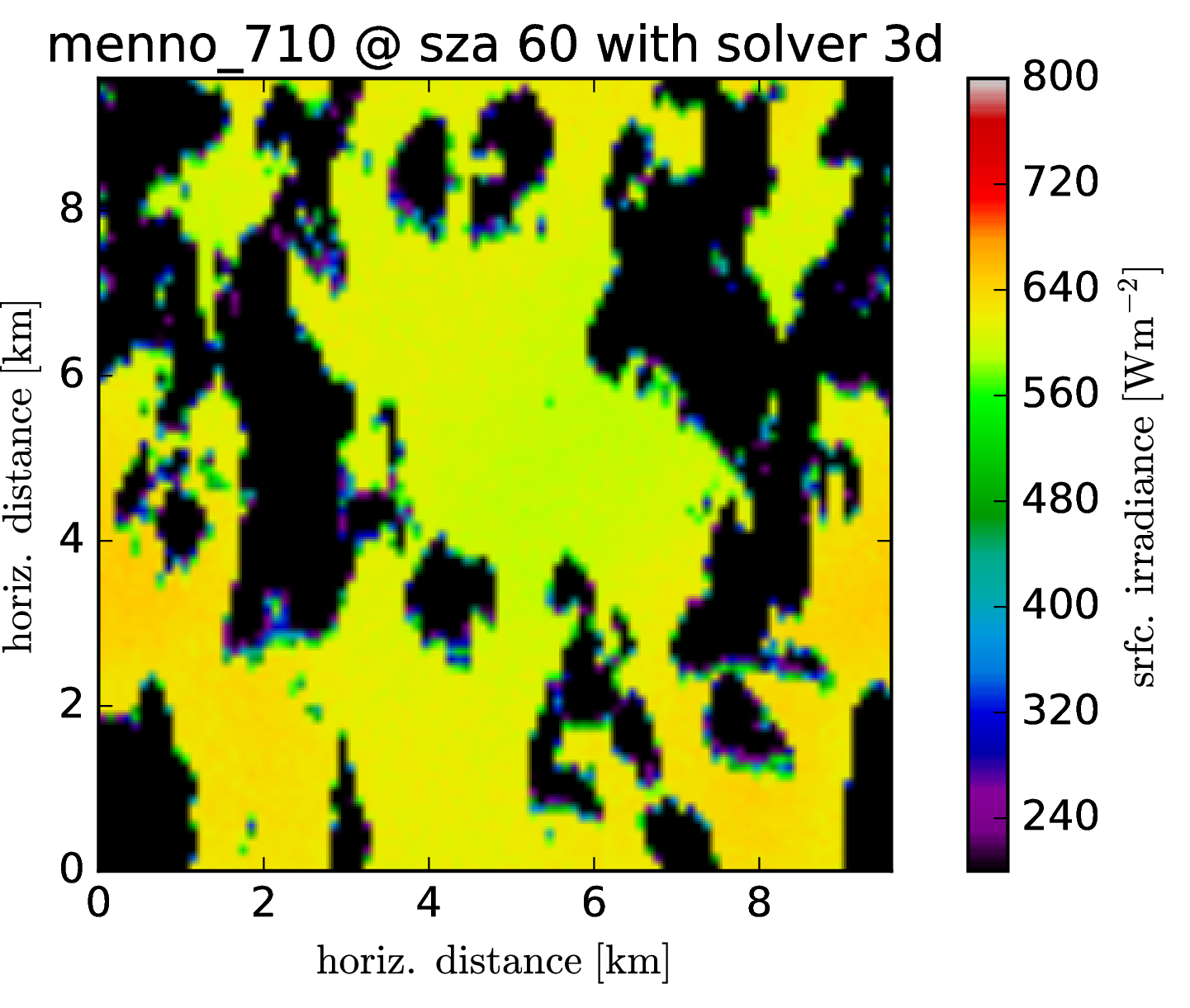
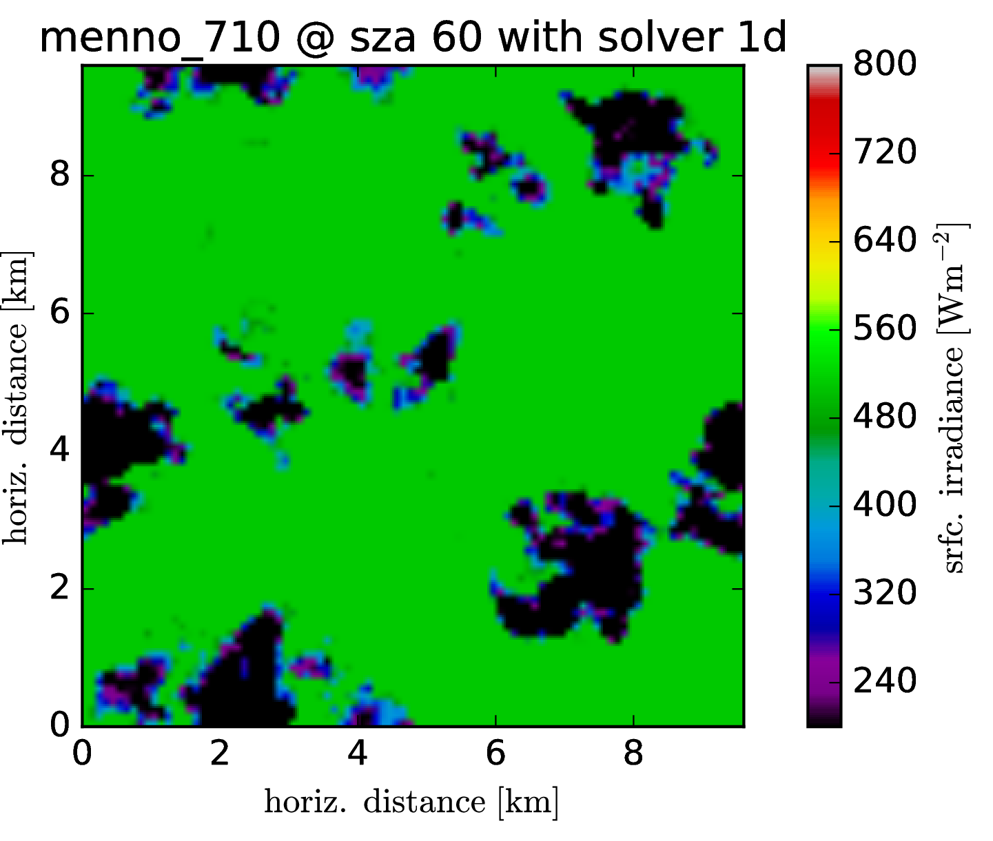
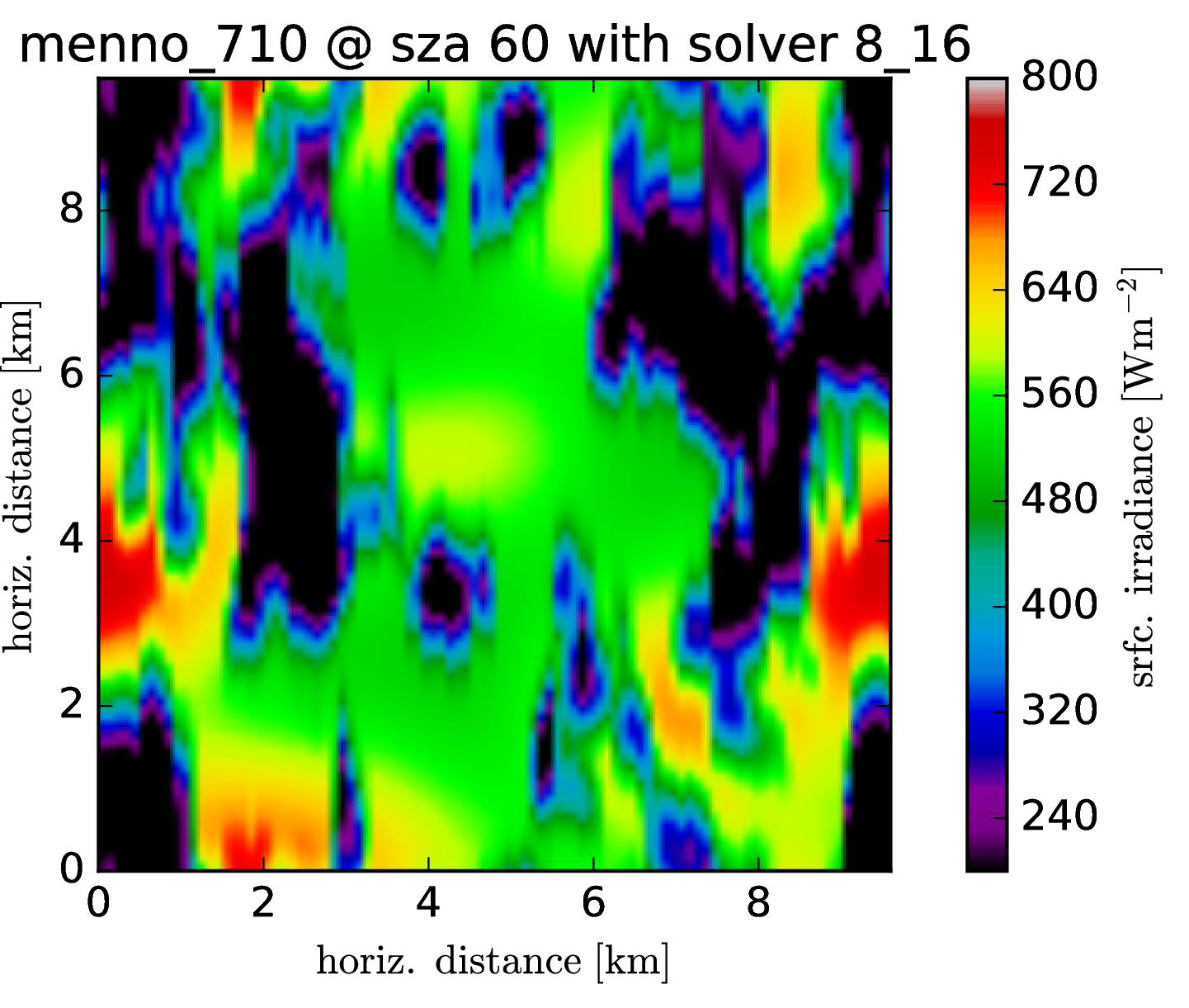
Srfc irradiance (direct + diffuse) SZA 60
Conclusions
I tried serveral more combinations of diffuse streams but all azimuthally averaged disections had close to no effect at all. It seems that the 16 stream variant gives consistently better results. I have not done a thorough analysis on the computational cost of the additional streams. Work-wise the overall memory footprint and work should scale with the number of degrees-of-freedom squared, so going from 10 to 16 increases the number of variables by a factor of 2.56. However, this is not necessarily the increase in time within the iterative solvers. It probably scales better but you have to try yourself. If it is worth it, I don’t know. You can try to rerun your simulations and check if it changes the argument considerably. Apart from that I think it may be a good idea to make the LES voxels more like a cube compared to these flat slabs. Is it possible to decrease the vertical resolution or increase the horizontal resolution (or both)? I think an aspect of say, 24m / 50m would probably give better results.
How to use it:
- Download the LookupTables from:
www.meteo.physik.uni-muenchen.de/~Fabian.Jakub/TenstreamLUT
- Get the newest master branch
- In your code, change the solver type from ‘t_solver_3_10’ or ‘t_solver_8_10’ to ‘t_solver_8_16’
Hope that works, if not, let me know.
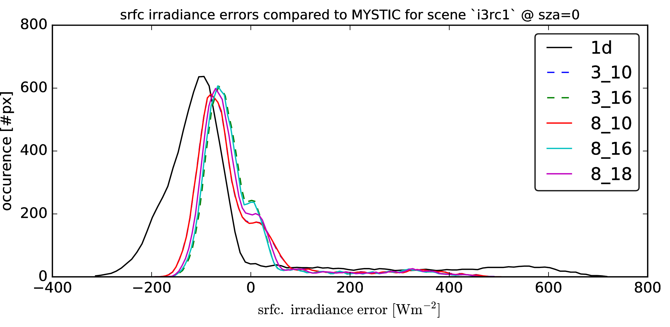
Comparison on the good old I3RC1 cumulus cloud fields
Just to make sure that mennos cloud field is not just a freak accident, lets do the same analysis on the by now well known I3RC1 cumulus cloud field which was use many times before for our benchmarking
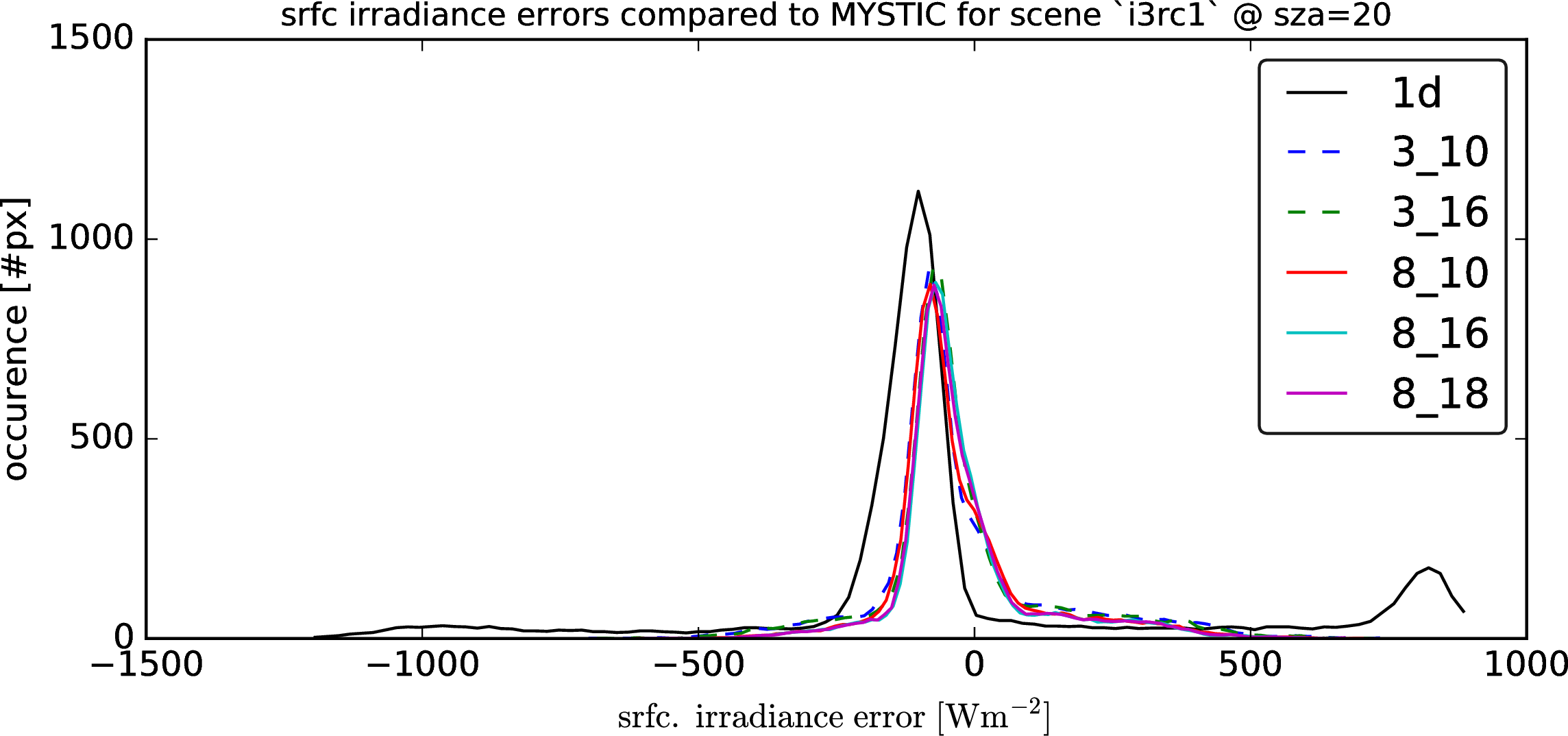
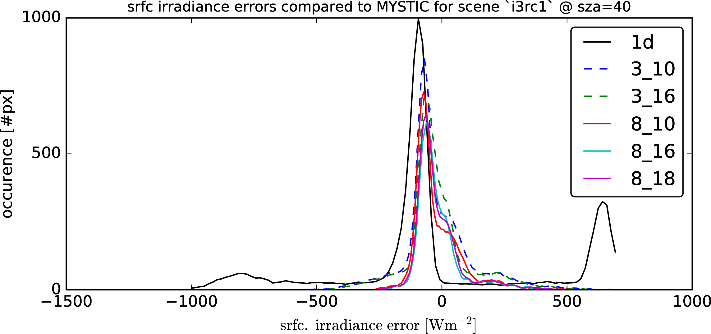
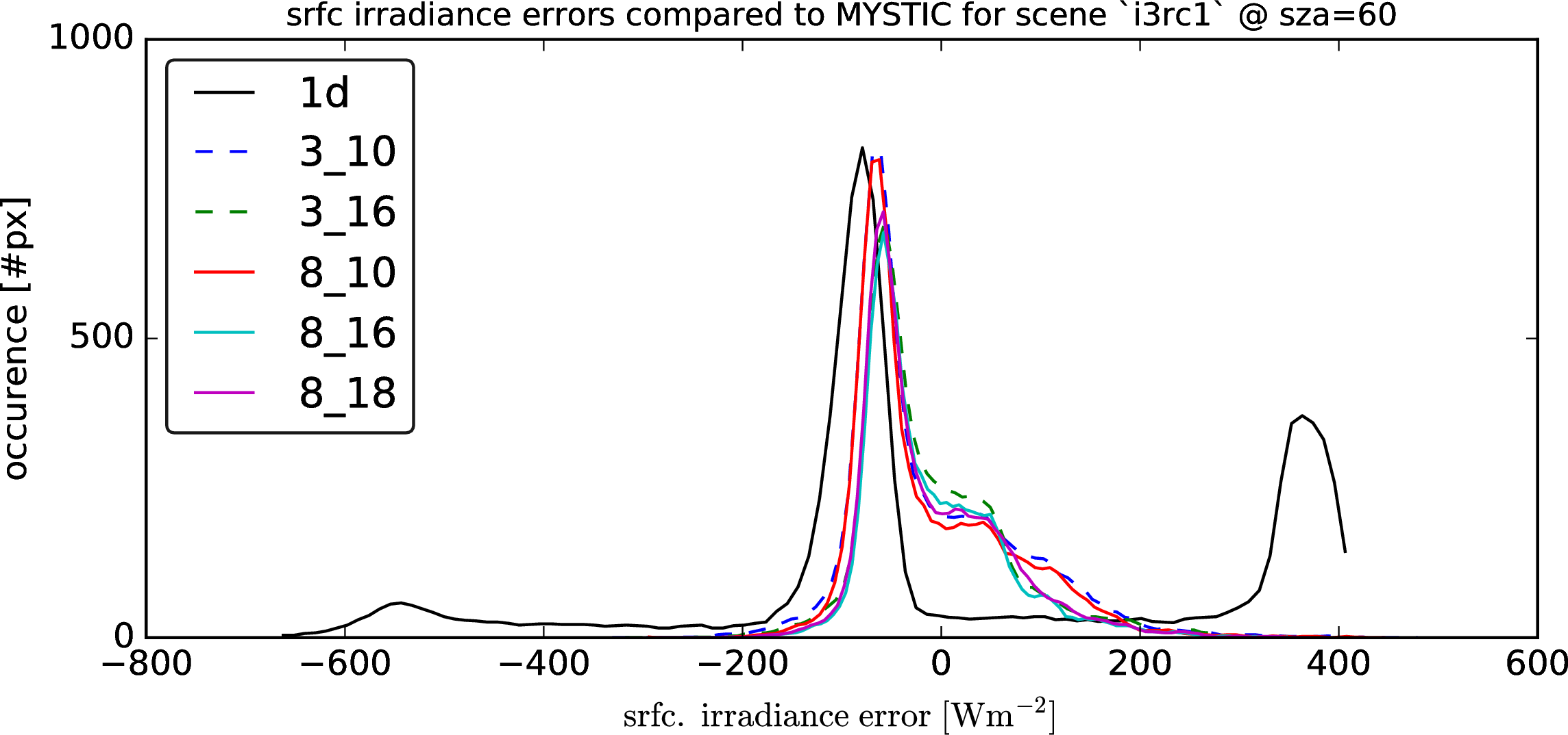
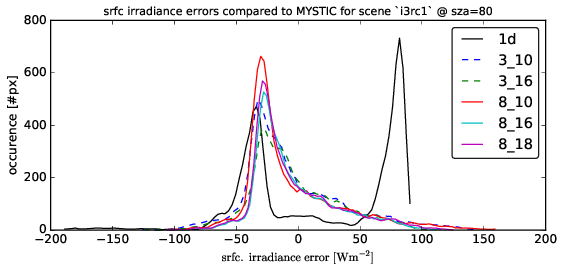
Following graphs show the error distributions for the total radiative flux at the surface for each solver compared to MonteCarlo benchmark simulations.
I.e. histogram( E_srfc(*) - E_srfc(3D MYSTIC) ) for several solar zenith angles
Max difference [W/m2]
max(abs(E_surface(*) - E_surface(MYSTIC)))
| SZA | 1D | 8_10 | 8_16 |
|---|---|---|---|
| 0 | 422 | 230 | 167 |
| 20 | 779 | 257 | 187 |
| 40 | 835 | 264 | 192 |
| 60 | 547 | 231 | 149 |
| 80 | 132 | 109 | 69 |