Lectures on Tropical Meteorology
Chapter 7. Steady and transient forced waves
We consider now a range of specific situations in which waves are excited in the equatorial wave guide. We begin with an analysis of steadily forced waves with application to understanding the structure of the Walker circulation and go on to study transient waves generated by tropical convection, or by middle latitude weather systems.
7.1 Response to steady forcing
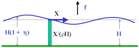
Consider a homogeneous ocean layer of mean depth H forced by a surface wind stress X = (X, Y ) per unit area. We assume that, through the process of turbulent mixing in the vertical, this wind stress is distributed uniformly with depth as body force X/(ρH) per unit mass.
|
Suppose that there is also a drag per unit mass acting on the water, modelled by the linear friction law -ru per unit mass. Then the equations analogous to (x.21) and (x.22) are
The continuity equation analogous to (3.23) takes the form

where E may be interpreted as an evaporation rate (i.e. rate of mass removal) and rη with r > 0 represents a linear damping of the free surface displacement. In the atmospheric situation, a positive/negative evaporation rate is equivalent to the effect of convective heating/cooling (see Chapter 6) and the damping term represents Newtonian cooling due, for example, to infra-red radiation space. Although formally obtained for a shallow homogeneous layer, we have shown that these equations apply for each normal mode, but with a value of appropriate to that mode. Also, the magnitude of the forcing is then determined by expanding the forcing function in normal modes.
As before, Eqs. (6.1)-(6.3) can be written as a single equation for v, i.e.
Note that leading terms involve only x derivatives, i.e. in the case of small friction (r → 0), this equation reduces to

which may be integrated with respect to x to give

When E = 0, this is Sverdrup's formula (see DM, Ch. 6).
7.1.1 Zonally-independent flow
In this case, (∂/∂x = 0) and Eq. (6.4) reduces to

a factor r has been cancelled. This formula is valid on an f-plane, or on an equatorial β-plane, where f = βy. In the latter case, solutions are possible in terms of parabolic cylinder functions of order ½ (see Gill 1982, p467).
|
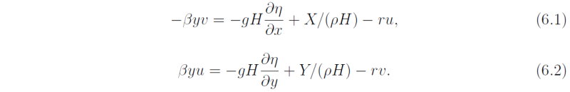
The upper panel of Fig. 2 shows the variation of surface elevation (or pressure perturbation p') for evaporation (or heating) concentrated along the line y = LE, the equatorial Rossby length. The variation of f is manifested in a slower fall off in pressure on the equatorial side of the evaporative sink. When the solutions are applied to baroclinic motions in an incompressible atmosphere of constant buoyancy frequency N with a "rigid lid" at some height, the baroclinic modes have a sinusoidal vertical structure (see section 5.8). The "gravest" mode (i.e. the one with the largest vertical scale) is a sine of height with half-wavelength spanning the depth. If diabatic heating is applied with this distribution in the vertical, only the gravest mode is excited and the equations are the shallow-water equations with heating replacing the evaporation term. The lower panel of Fig. 2 shows the corresponding meridional circulation produced by such heating concentrated on the line and is obtained by attaching the appropriate vertical structure to the solutions of (6.7). This is a type of Hadley circulation that is generated by a line source of heating such as occurs along the ITCZ. Rising air is found only in the heating zone. Most air is drawn in form the equatorial side, so that the most pronounced circulation is on this side. The pressure curve shows how the surface pressure varies with such solution.
7.1.2 Zonally-dependent flow
Gill (1982, p469) explains how to construct a solution to Eq. 6.4 for the more general case of a localized heating covering a restricted range of longitudes and similar to that which obtains in the atmosphere in July. If the equatorial Rossby length LE is taken to be about 10o of latitude, the solution shown in Fig. 3 with L = 2LE corresponds to maximum heating at about 10o and covering 40o of longitude. According to Newell et al. (1974; see plate 9.1), the region of large heating in the atmosphere is concentrated as it is in Fig. 3, but with maximum at about 15o and with largest values between 90oE and 140oE longitude.
|
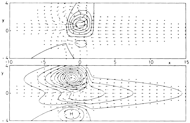
In the region of heating, Fig. 3a shows vertical motion and mainly northward velocities, although there is some distortion on the west side because of friction. The interpretation is that ascent associated with the heating causes vortex stretching and thereby to the generation of cyclonic vorticity. Thus the fluid particles tend to move polewards in order to keep their relative vorticity small. The only wave that can propagate eastwards from the forcing region is a Kelvin wave, so that the region x > L (corresponding to the Pacific Ocean if the model is applied to the effect of forcing over Indonesian longitudes) shows motion with characteristic features of the Kelvin wave, namely, flow parallel to the equator and symmetric about the equator.
The winds are easterly toward the heat source and decay eastward at the rate r/c per unit distance. Physically, the decay process represented by r (Geisler, 1981) appears to be "cumulus friction" due to momentum transfer between levels through cumulus activity. Long planetary waves can propagate westward from the forcing region, but they decay faster than the Kelvin waves and thus cover a smaller area. They include meridional motion, so the equatorward return of the air moving poleward in the heating region is found to the west. The result is a cyclonic center on the west flank of the heating region. (Comparisons can be made with the observed 850-mb flow shown in Fig. 1.11.) Solutions with similar properties were found by Webster (1972), who obtained numerical solutions with a two-layer model for perturbations on a zonal flow, and Matsuno (1966), who obtained solutions for forcing periodic in x. Solutions of the shallow-water equations with friction on a sphere, as obtained by Margules (1893), show Similar characteristics also.
The upper panels of Fig. 4 show the zonally averaged flow, exhibiting a strong Hadley cell with rising motion in the latitude of maximum heating. Equatorial motion is associated with easterlies and poleward motion with westerlies. This is due to conservation of angular momentum and the fact that, in a linear formulation, the fluid "remembers" only the angular momentum from the latitude where it has just been. Thus the zonal velocity changes sign on crossing the equator. The lower panel of Fig. 4 shows the meridionally averaged circulation, which is due only to the part of the forcing that is symmetric about the equator. Rising motion is found over the longitudes of the heating region, and sinking elsewhere. The circulation corresponds with the Walker circulation discussed in Chapter 1.
|
7.2 Response to transient forcing
The low-latitude atmospheric response to transient forcing can be studied also using the equatorial β-plane model described in this chapter. Silva Dias et al. (1983) used such a model to investigate the atmospheric response to localized transient heat sources, which crudely simulate convective bursts in the tropical region. The equations of motion are similar to Eqs. (5.73), (5.74) and (5.78), but include forcing terms on the right-hand sides similar to Eqs. (6.1) - (6.3). The reader is referred to the original paper for details of the formulation, which uses ln p as vertical coordinate rather than the actual height as used here.
Silva Dias et al. (1983) study the case where a heat source is added to Eq. (5.78) with the form:

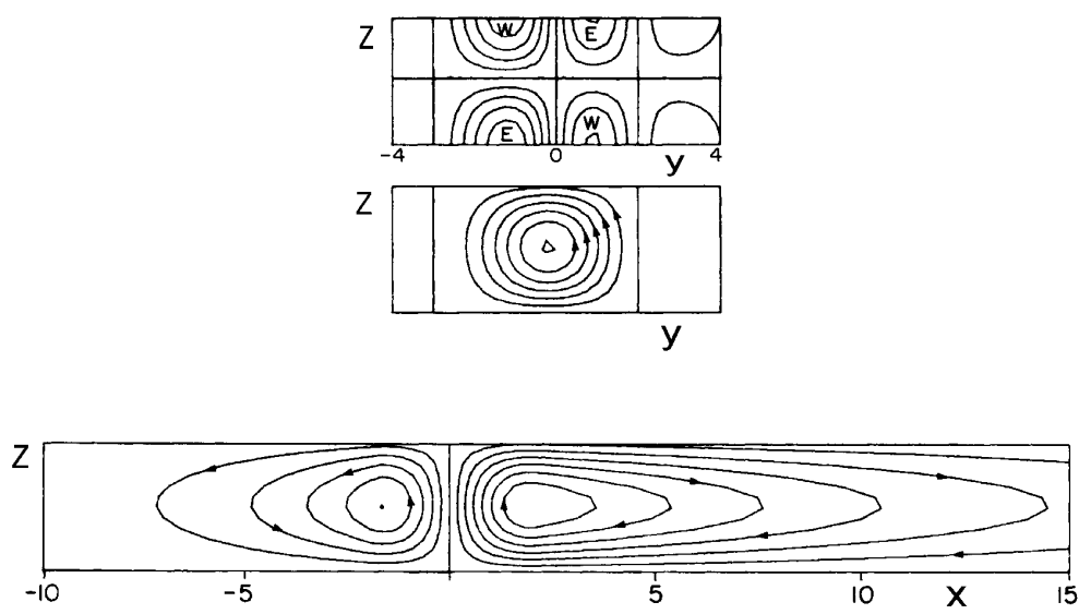
This heat source is centred at a distance y0 from the equator and has e-folding radius a. The time dependence χ(t) is given by

where α is a nondimensional parameter that characterizes the rapidity of the forcing (see Fig. 5).
|
The forcing is a maximum when t = 2/α, which corresponds to about 4 h for α = 4 and about 12 h for α = 4/3, using the time scale for the first internal mode in the calculations. The total heating is independent of α since

and it is independent of y0 since

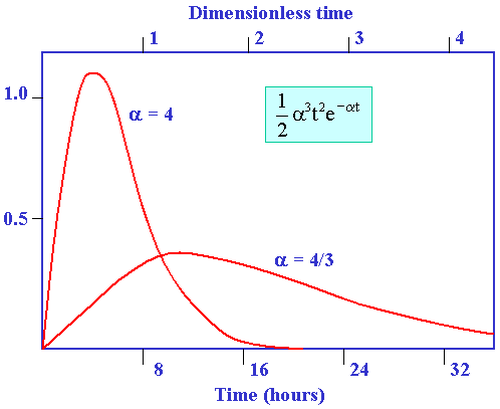
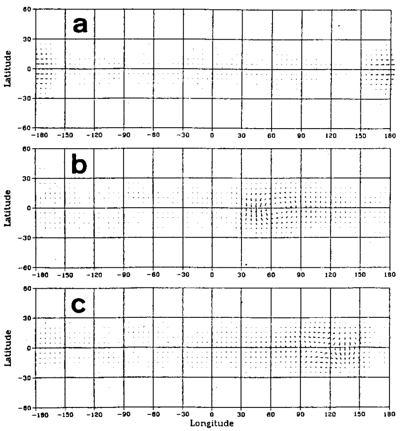
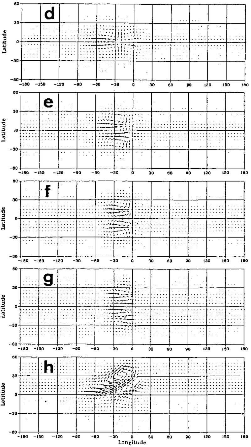
Silva Dias et al. (1983) used transform techniques to solve the equations. Here we summarize some of the key results. Figure 6 shows the wind and geopotential fields for the case α = &frac43;, a = 0.5 and y0 = -0.8 at t = 2, 4, 6 and 8 nondimensional units. Also shown is the contribution to the total field from the Kelvin waves (panels b), mixed Rossby-gravity waves (panels c) and Rossby waves (panels d). The wind and geopotential fields are equally scaled. For the internal mode corresponding to c = 51 m s-1 the dimensional time scale [T] is 8 h and the spatial scale [L] is ≈ 1500 km. Using this scaling, the e-folding radius of the thermal forcing is then 750 km and the latitude of the forcing is 11oS. As can be seen in Fig. 7, when a = 4/3, the forcing is a maximum at t = 1.5 nondimensional units and becomes negligible after t = 6 nondimensional units which correspond to t = 12 h and t = 48 h respectively.
(a) 16 h (left), 32 h (right)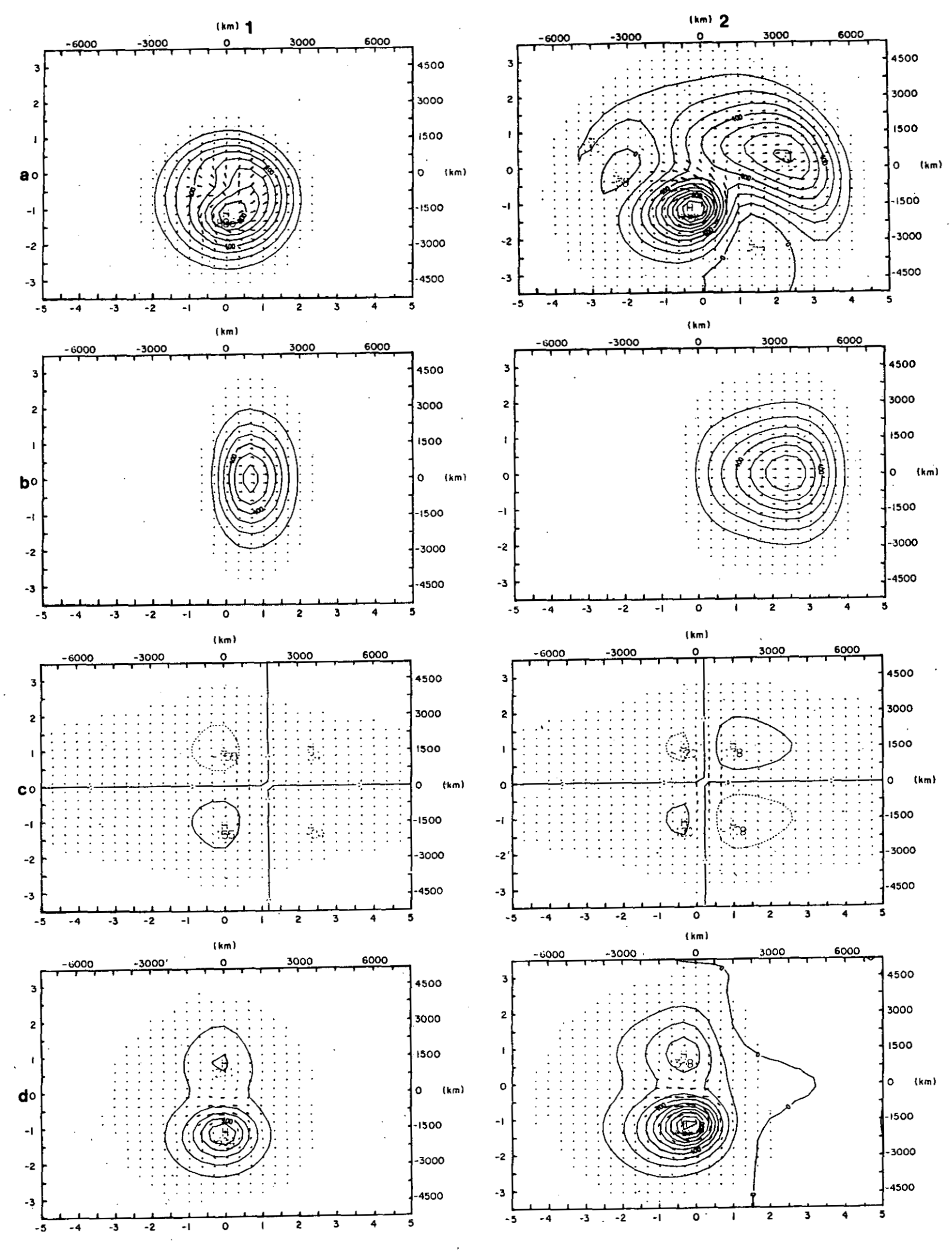
|
(b) 48 h (left), 64 h (right) 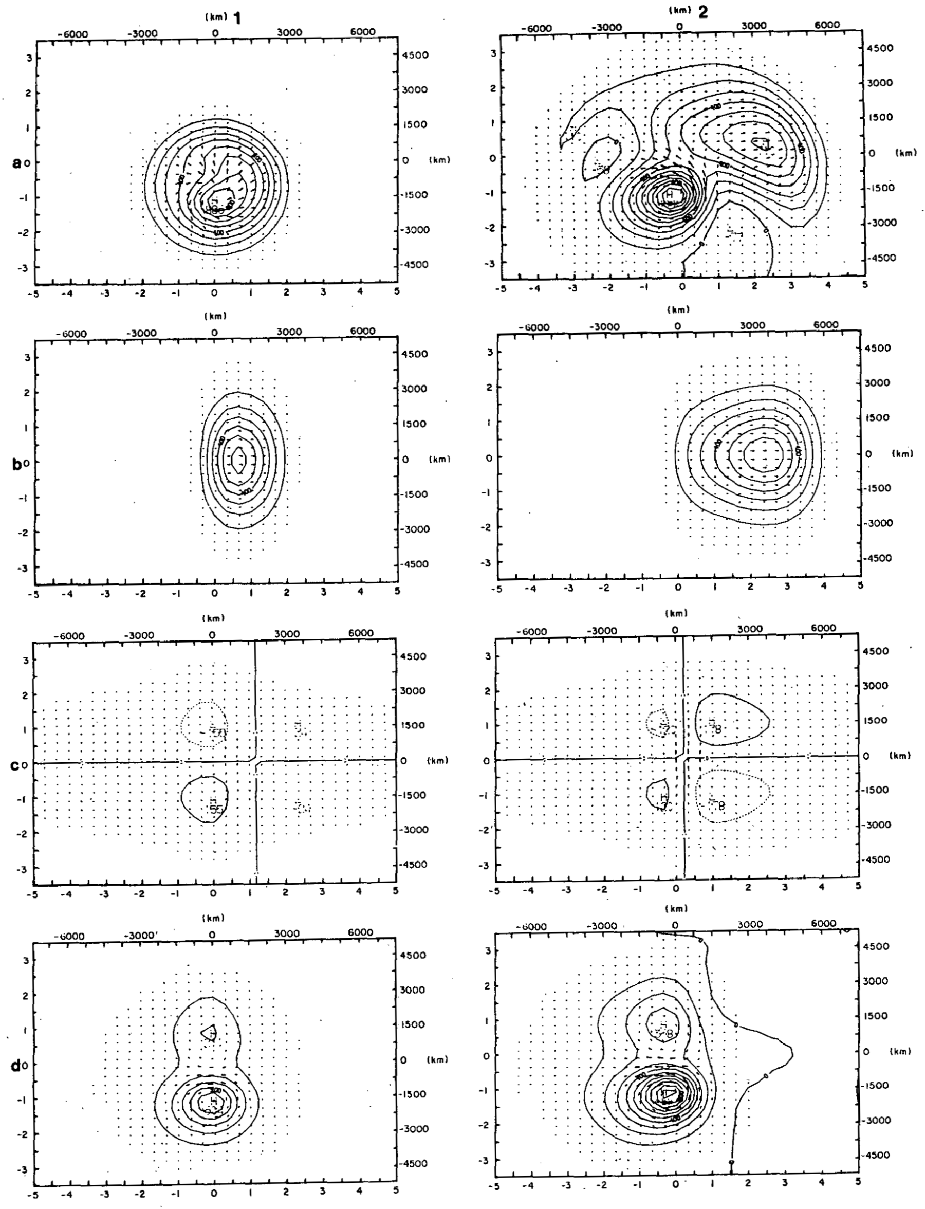
|
The total flow fields (top panels of Fig. 6) show many interesting features.
At t = 16 h (top row, left column) the high-pressure centre that developed in response to the forcing is displaced slightly south of the maximum forcing. Also noticeable is the asymmetry of the response. There is a strong cross-equatorial flow with the maximum wind speed in the neighbourhood of the equator. The flow pattern becomes more geostrophic as the latitude increases in agreement with the larger Coriolis parameter.
At t = 32 h (second left column) the forcing has decreased to 25% of its maximum intensity and the flow pattern is becoming more geostrophic although the cross-isobaric flow is still intense near the equator. At this time there are several features that deserve attention:
(i) the southerly and southeasterly flow on the northeast side of the anticyclone have become more intense,
(ii) the centre of the anticyclonic circulation is now displaced west of the maximum forcing,
(iii) a trough is beginning to develop east of the anticyclonic circulation,
(iv) westerlies have developed along the equator with maximum wind speed at x = 3000 km and maximum pressure perturbation displaced slightly towards the Northern Hemisphere and
(v) the flow across the equator now has an anticyclonic curvature in the Northern Hemisphere.
At t = 48 h and t = 64 h the above characteristics tend to become more evident except that the cross-equatorial flow north of the main high pressure has decreased and a new region of cross equatorial flow with a northerly component has developed between x = 1500 km and x = 4500 km. By t = 48 h the forcing has decreased to 4% of its maximum value and the whole flow pattern is slowly dispersing. The main anticyclone is becoming elongated toward the west and a sharp east-west geopotential gradient is forming between the low centred near x = 1500 km and the main high. Accordingly, strong winds are also observed in this region. Also noticeable is the rapid eastward drift of the circulation pattern discussed in item (iv). A comparison of panels (a) and (b) in Fig. 6 shows that this circulation pattern is associated with the Kelvin wave contribution. Thus, the cross-isobaric flow observed on the northeast quadrant of Fig. 6.6a at t = 16 h moves eastward and propagates as a nondispersive wave group.
At first it may appear that the Kelvin waves in Fig. 6 are exhibiting a dispersive behaviour since the initially narrow disturbance at t = 16 h becomes elongated at later times. However, this feature is due to the continual generation of Kelvin waves while the forcing is active. After t = 48 h when the forcing becomes negligible the Kelvin wave group propagates eastward without changing shape.
The contribution from the mixed Rossby-gravity waves shown in Fig. 6c is small, but is responsible for certain features of the total flow field. The mixed Rossby-gravity waves have a westward phase speed, but propagate energy eastwards. This feature can be seen in panels (c) of Fig. 6 as a successive eastward reinforcement of the geopotential and wind maxima. Comparing panels (a) and (c) in Fig. 6 at t = 48 h and t = 64 h shows that the northwesterly flow at the equator between x = 1500 km and x = 3000 km, and the lowering of the geopotential near y = -1500 km and x = 1500 km in the total solution, are associated with the mixed Rossby-gravity waves. The formation of this trough east of the main anticyclone is caused also partially by the eastward dispersion of short Rossby waves which can be seen by comparing Figs. 6a and 6d at t = 64 h. The formation of the low geopotential region at x = 3000 km and y = 2000 km, which is most evident at t = 64 h, is primarily related to the mixed Rossby-gravity waves also with some contribution from the shorter Rossby waves.
The panels in row (d) of Fig. 6 show the contribution to the total solution from the Rossby waves. Comparing Figs. 6d and 6a after t = 32 h shows that the high geopotential configuration which appears in the Northern Hemisphere is a manifestation of the Rossby waves. This high pressure is generated in response to the heat source and migrates westward in the early stages of the transient solution. The pattern continues to move westwards after the forcing becomes negligible. This evolution in time can be explained by the group velocity of Rossby waves, the sign of which can be deduced from the dispersion curve for these waves shown in Chapter 6, Fig. 9. The zonal component of the group velocity is given by -∂ν/∂μ, which is the slope of the dispersion curve. Since the slope changes sign (except for m = 0), it is evident that the group velocity is eastward for short Rossby waves and westward for long Rossby waves. Thus, the westward elongation of the geopotential field in Fig. 6d is due to the dispersion of long Rossby waves and the intensification of the east-west gradient of the geopotential field east of the main high is a result of the eastward dispersion of short Rossby waves.
The appearance of a stronger meridional flow at the longitude of maximum forcing is predictable also from the dispersive properties of Rossby waves since short Rossby waves are almost nondispersive and have more kinetic energy in the meridional than in the zonal component of the wind (Longuet-Higgins, 1964). The strong easterly flow along the equator and the predominately symmetric pattern that develops in panels (a) of Fig. 6 can be associated with the m = 1 Rossby mode. This particular mode is expected to have a large contribution to the solution because of its horizontal similarity with the forcing function.
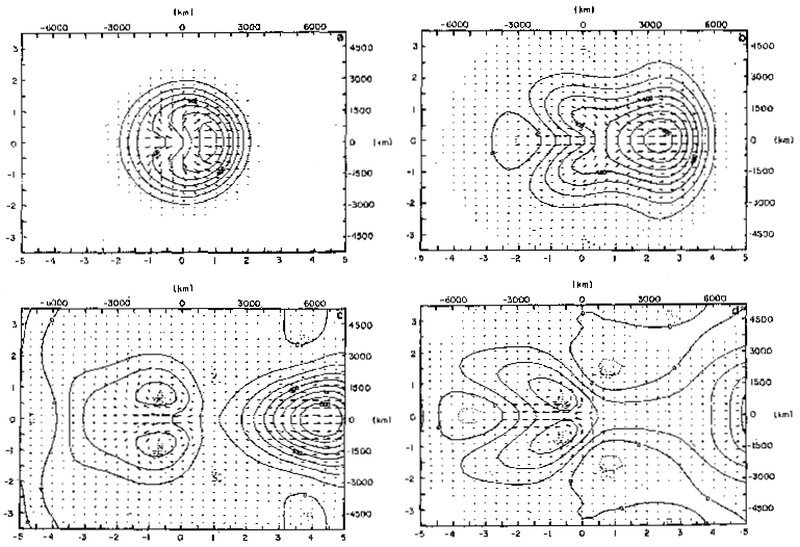
Figure 7 shows the total wind and geopotential fields for the case when the heat source discussed previously is centred at the equator (α = 4/3, a = 0.5 and y0 = 0). As discussed in section 3 of Silva Dias et al. 1983), more of the energy of the final adjusted state is in the Kelvin modes than in the Rossby modes (see their Fig. 3d). This explains the large amplitude configuration that moves rapidly eastwards in Fig. 7. Since the forcing is symmetric about the equator, the initial outward spreading mass builds up two high-pressure centres, which are separated by an equatorial trough. During the initial development, (t = 16 h) it is evident that the mass tends to flow primarily along the equator with the streamlines curving toward the poles and away from the heat source. After the Kelvin waves propagate toward the east, the symmetric Rossby waves, which remain in the region of the heat source slowly, disperse.
|
The fields shown in Fig. 7 differ somewhat from the case where the equatorial heat source is stationary in time as discussed in Chapter 6, section 6.8. The stationary case shows a zone of upper-level westerlies to the east of the forcing which is much more extensive than the zone of upper easterlies to the west of the forcing. Gill pointed out that the the relative sizes of the east-west circulations is explained by the continual generation of the Kelvin waves by the stationary forcing, coupled with the large eastward group velocity of the Kelvin waves compared to the westward group velocity of the long Rossby waves. In the transient case shown in Fig. 6 the forcing becomes negligible after t = 48 h so that very little Kelvin wave energy is being generated. The previously generated Kelvin waves propagate to the east leaving only the upper-level easterly flow to the west of the forcing which is associated with the slower propagating Rossby waves.
The simulations presented in Figs. 6 and 7 show the response of the model to a transient heat source centred at two different latitudes.
For comparison, Fig. 8 shows 200 mb FGGE maps at 0000 GMT 6 Feb. and for 9-12 Feb. 1979 prepared by the European Centre for Medium Range
Weather Forecasting (ECMWF). During a period of 2-3 days before 6 Feb., the Bolivian high was not well developed and the main synoptic feature
in the equatorial region of South America was an upper-level cyclone off the northeast coast of Brazil. This is the type of upper low studied
by Kousky and Gan (1981). After 6 February, the anticyclonic circulation began to organize and during the period 9-12 Feb. (Figs. 6b-6e), the
Bolivian high was again established. On 10 Feb. there was a strong crossequatorial flow at 50oW that turned and became a westerly
flow at about 30oW.
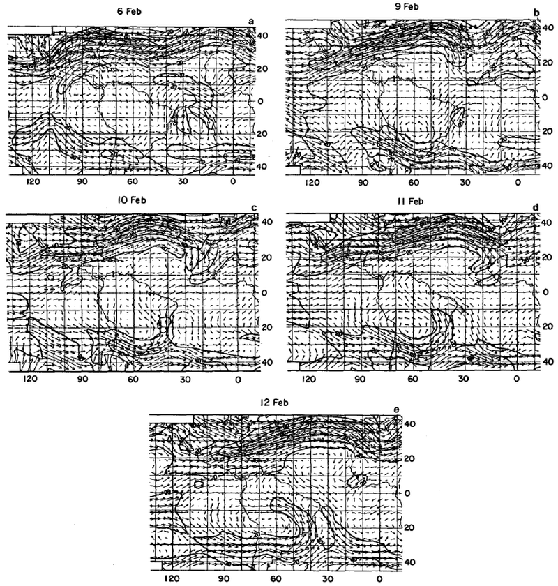
The most significant change occurred between 10 and 11 Feb. with the sudden increase in speed of the southerly component between the centre of the Bolivian high and the upper trough off the northeast coast of Brazil. On 10 Feb. the cross equatorial flow was well established and the anticyclonic circulation was developing in the Northern Hemisphere as a result of the change in sign of the Coriolis parameter. The trough off the northeast coast of Brazil was elongated and tilted northwest to southeast.
On 12 Feb. the Bolivian high was stretched in the east-west direction with the flow more zonal in the vicinity of the equator and with the wind stronger in the eastern and northeastern sectors of the Bolivian high.
The model results shown in Figs. 6 and 7 reproduce some of the transient aspects of the Bolivian high. As noted by Virii (1981), a southerly component of the wind dominates over most of the region east and north of the Bolivian high. This is evident in the 9-12 Feb. period shown in Fig. 8, and can also be seen in the model results shown in Fig. 6a. The model results indicate that initially cross-equatorial flow dominates north of the forcing and that it is replaced by easterly flow as the forcing becomes negligible. A similar feature can be seen in Fig. 8.
Between the 9th and 10th, cross-equatorial flow is established north of the Bolivian high which turns to easterly flow by the 12th. Virgi (1981) observed also maximum mean wind speeds greater than 10 m s-1 and exceeding 25 m s-1 on certain days within the latitudinal band between 5o and 10oS. The model results indicate that this equatorial easterly jet appears when the Rossby wave component of the solution becomes dominant after the forcing becomes negligible.
As is shown in Fig. 8, the Bolivian high has become elongated in the east-west direction and has maximum winds to the northeast by 12 Feb. These features are seen also in the model (Fig. 6). The westward elongation of the main high is caused by the westward dispersion of long Rossby waves while the sharp geopotential gradient and large wind speeds to the east are caused by the eastward dispersion of short Rossby waves.
The model results show also the formation of a trough east of the main high cell, The modal decomposition shown in Fig. 6 indicates that this is a manifestation of the eastward dispersion of the Rossby and mixed Rossby-gravity waves emanating from the source region. A similar trough east of the Bolivian high can be seen in Fig. 8 which gradually sharpens up and acquires a northwest-southeast tilt between the 9th and 12th. The anticyclonic flow which developed in the Northern Hemisphere in the model also has its counterpart in the observed flow shown in Fig. 8.
7.3 Wintertime cold surges
During the northern winter, the East Asian continent is dominated by a strong surface high over Siberia and northern China. Radiative cooling and persistent cold air advection throughout the troposphere maintain a layer of very cold air over the frozen land. The Tibetan plateau to the southwest restricts the movement of this cold air mass and contributes to the buildup of the surface high. A strong baroclinic zone exists between this cold continental air mass and the warm tropical air mass to its south. A manifestation of this strong baroclinic zone is the steady jet stream over the coast of East Asia. The continental anticyclone fluctuates in strength in response to midlatitude synoptic developments.
The passage of a deep upper trough in the midlatitudes often triggers intense anticyclogenesis over central China and cyclogenesis over the East China Sea. As the pressure gradient across the East China coast tightens, cold air bursts out of the continent toward the South China Sea and a cold surge is initiated. In a normal season, cold surges may occur at intervals of several days to about two weeks.
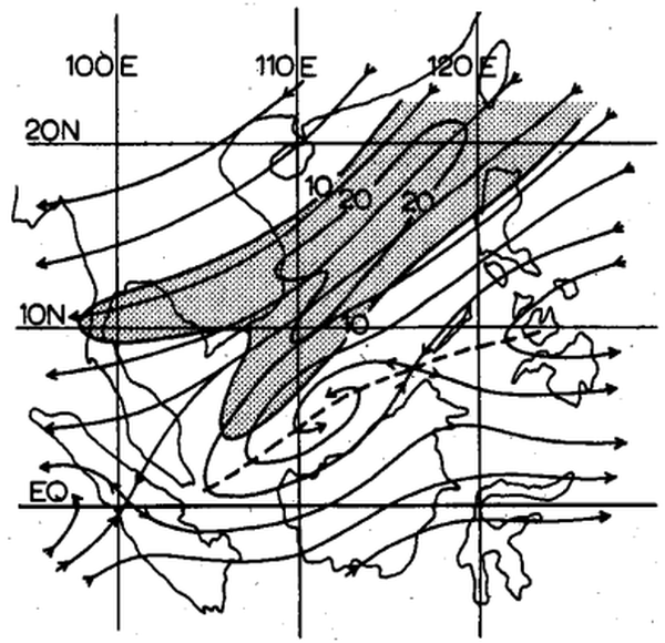
In the midlatitudes, a surge arrives with a steep rise of surface pressure, a sharp drop of temperature, and a strengthening of northerly winds. The cold front leading the surge sometimes brings stratus and rain, but a strong surge is generally associated with subsiding motions that lead to a clearing of weather (Ramage 1971). Although normally the front associated with the surge cannot be followed southward of about 20oN, the surge propagates equatorward in a dramatic fashion. As a vigorous surge reaches the South China coast, northerly winds freshen almost simultaneously several hundred kilometers to the south, far beyond the region where the winds could have pushed the front (Ramage 1971; Chang et al. 1979). A belt of strong northeasterly winds forms within 24 h off the South China and Vietnam coasts and leads to a strengthening of a quasi-stationary cyclonic circulation embedded in an eastnortheast -westsouthwest-oriented equatorial trough just north of the Borneo coast (see Fig. 9).
|
In the equatorial region south of East Asia lies the maritime continent of Malaysia and Indonesia. During winter, extensive deep cumulus convection over this region supplies a large amount of latent heat to the atmosphere and is believed to be one of the most important energy sources that drive the winter general circulation (Ramage 1971). From the results of a series of observational studies, Chang et al. (1979) and Chang and Lau (1980, 1981) suggested that this equatorial convective heat source may interact with the cold surges from the north, resulting in modifications of both synoptic- and planetary scale motions. Their findings were supported by later studies (Chang and Lau 1982; Lau et al. 1983).
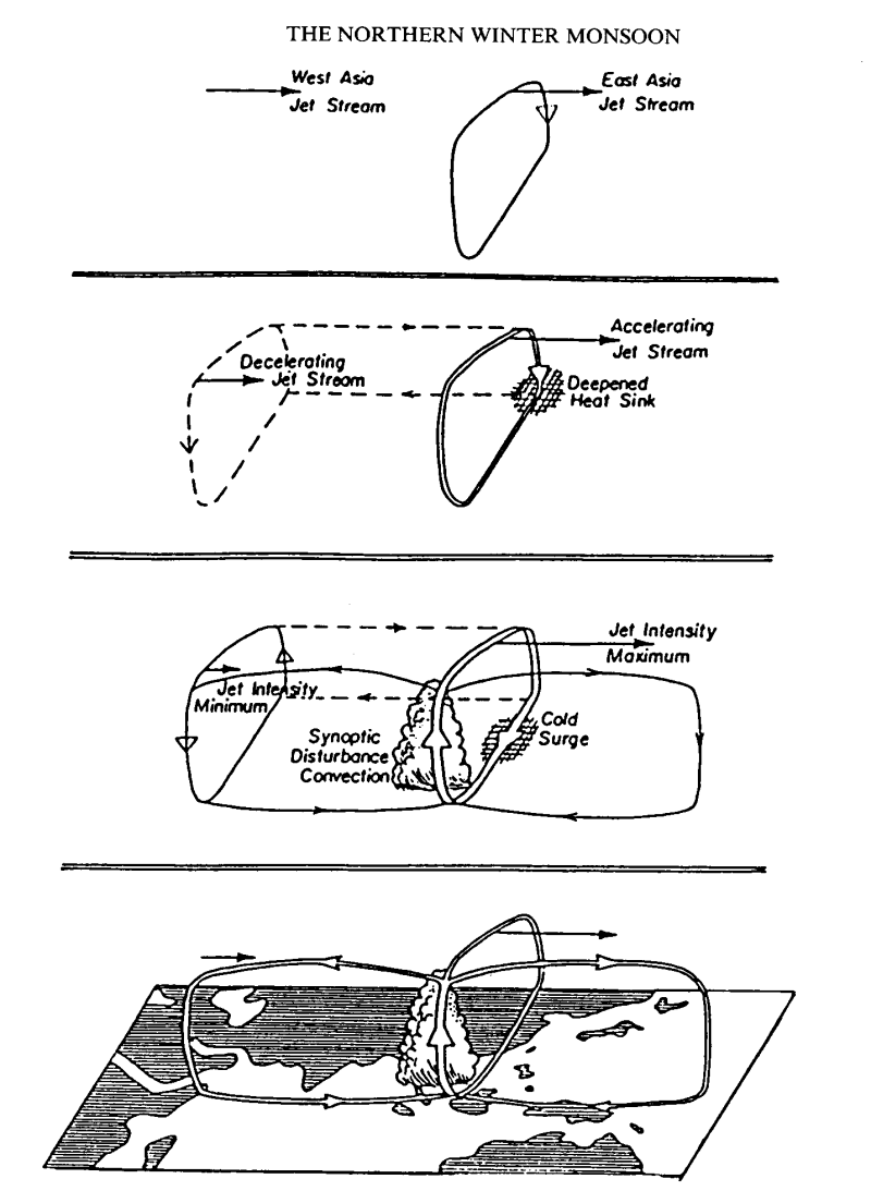
Chang and Lau (1980) summarized the sequence of events in the schematic diagram reproduced as Fig. 10. They noted that cold surges are often preceded by intense cooling over northern China. Such cooling appears to be due to the advection of polar air behind upper-level troughs that move rapidly eastward and deepen over northern Japan. The sinking cold air over the continent accelerates the East Asia local Hadley cell. Almost simultaneously, the east Asian jet stream centered over Japan intensifies due to the Coriolis acceleration by the ageostrophic southerly flow of the enhanced Hadley circulation.
|
There is a weakening also of the west Asian jet stream after a small time lag, possibly due to an induced reverse local Hadley-type circulation, as indicated in the Fig. 10. As a surge arrives over the equatorial South China Sea, the existing synoptic-scale convective systems flare up and warm the tropical atmosphere by release of latent heat. The upper-level outflow from the South China Sea convection region spreads mainly east and west, driving two Walker circulations. A smaller part of the outflow returns poleward, maintaining the enhanced Hadley circulation. In this panoramic view, cold surges are seen to be an important link in a complicated chain of midlatitude tropical and equatorial east-west interactions. Through these interactions, the effect of an intense baroclinic development over the east Asian continent is spread deep across a wide equatorial belt ranging from East Africa to the mid-Pacific Ocean.
Later studies indicated that a cold surge may even have influence over atmospheric motions in the Southern Hemisphere. Williams (1981) described a case of such cross-equatorial influences. About three days after a surge crossed the South China coast, he observed a slow pressure rise over western Indonesia. As if accelerated by the east-west pressure gradient, westerly winds strengthen and convective systems were observed to develop in the southern equatorial region and drift eastwards at a speed of 10 m s-1. His observation was supported by Lau (19S2) who found similar eastward-moving systems in a composite study of satellite imagery. Lau (1982) investigated also the meridional symmetry of such eastward-propagating cloud patterns and, with reference to the theory of Lim and Chang (1981) and Lau and Lim (1982), identified them to be Kelvin wave responses to cold surges.
Ref to Love
Davidson et al. (1983) presented some data that suggested a possible relation between cold surges and the onset of the Australian
monsoon (Fig. 11). In Fig. 11a, the strong northerly winds over the South China Sea show that a cold surge was in progress. Four days
later, the surge winds penetrated deep into this Southern Hemisphere, and the Australian monsoon became established (Fig. 11b).
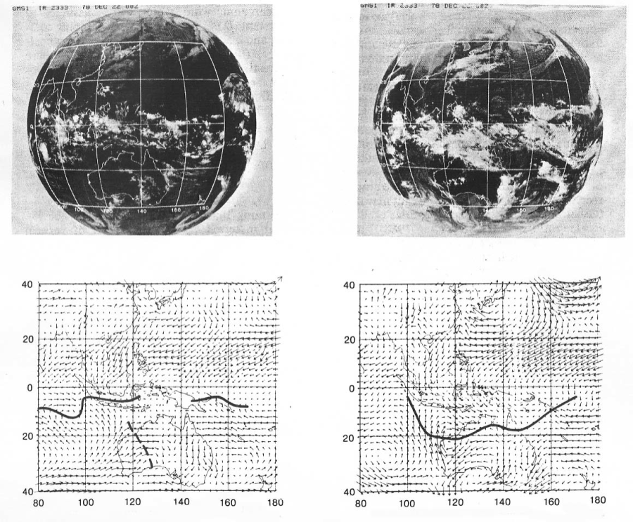
It may be noted that the extensive cloud system associated with the Australian monsoon onset was embedded within the belt of cross-equatorial flow. This observation and the overall flow pattern give one a strong impression that the Australian monsoon and the East Asia winter monsoon cold surges may not be independent events. Chang et al. (1985) presented also evidence linking the Northern Hemisphere cold surges to monsoon development in the southern hemisphere tropics. In a composite of the surface flow patterns for the southern summers of 1974 to 1983, they showed that the onset of the monsoon westerlies along 10oS in the Indonesian region is sometimes preceded by a significant strengthening of northeasterly monsoon winds that persists for three to four days. This wide range of processes related to the northern winter cold surges poses challenging questions to researchers in atmospheric dynamics. How does an intense midlatitude anticyclonic development give rise to strong northeasterly surge winds over the South China Sea, which often spread so rapidly southward as to give one an impression of near-simultaneous buildup? What are the mechanisms of interaction between the cold surge and tropical convective systems? Why is it that heating of the tropical atmosphere apparently enhances Walker circulations more than Hadley circulations? Is there a dynamical interpretation for the observed midlatitude-tropical and inter-hemispheric interactions?
Lim and Chang (1981) carried out calculations similar to those of Silva Dias et al. (1983) in an effort to understand the
northeasterly monsoon surges and associated tropical motions over southeast Asia during northern winter. They studied the
dynamical response of the tropical atmosphere to midlatitude pressure surges using again the linearized shallow-water equations
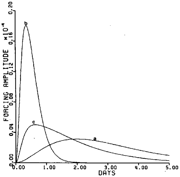
on an equatorial β-plane. The forcing is specified to have a Gaussian spatial distribution with a zonal scale corresponding to
approximately wavenumber 7 and a meridional scale of approximately 11o. It rises rapidly from zero to maximum within
one day or less and then decays slowly over 2-4 days (see Fig. 12).
The characteristics of the midlatitude-tropical interactions are clearly illustrated by the solution for τ = 15 ×
103 s, or about 4 h (Fig. 13).
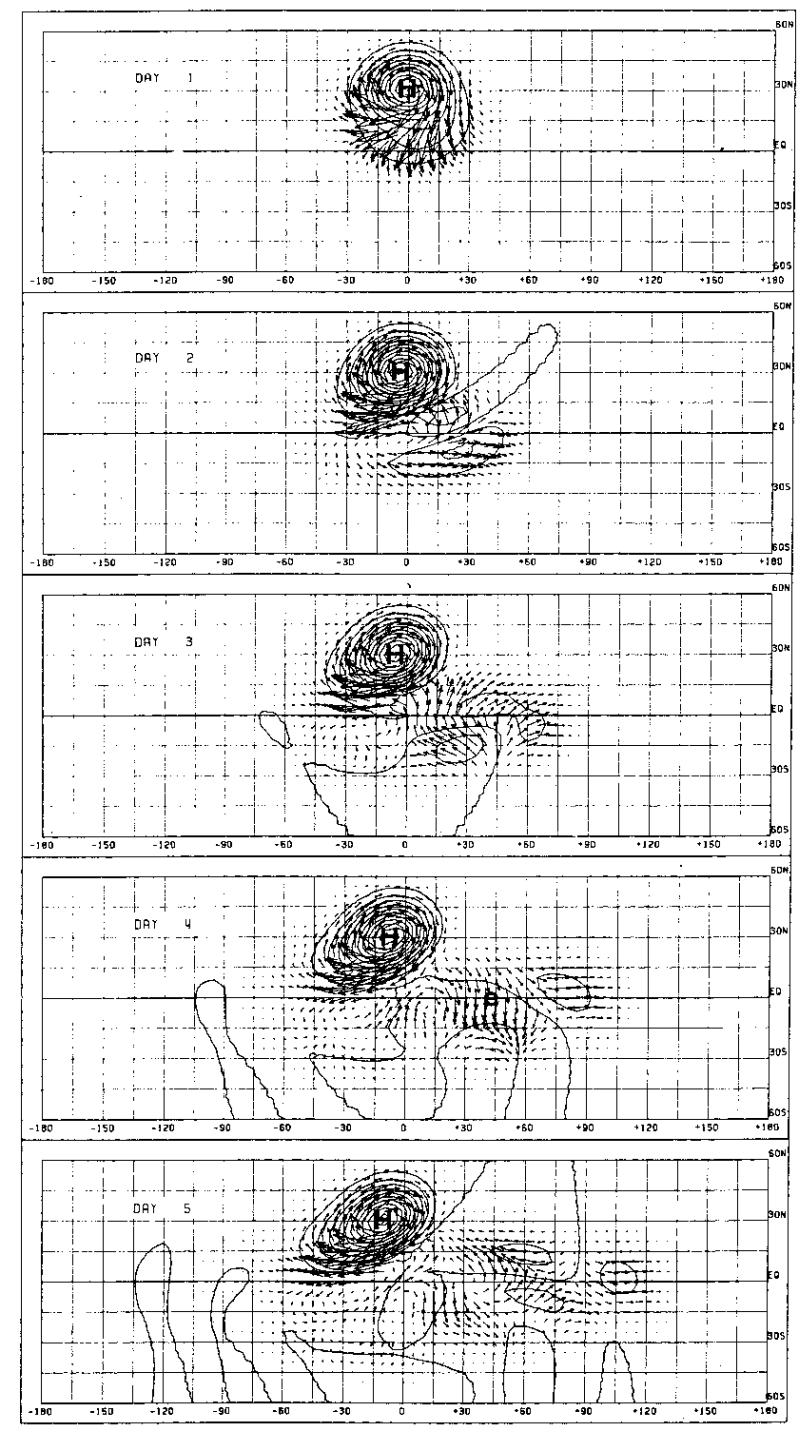
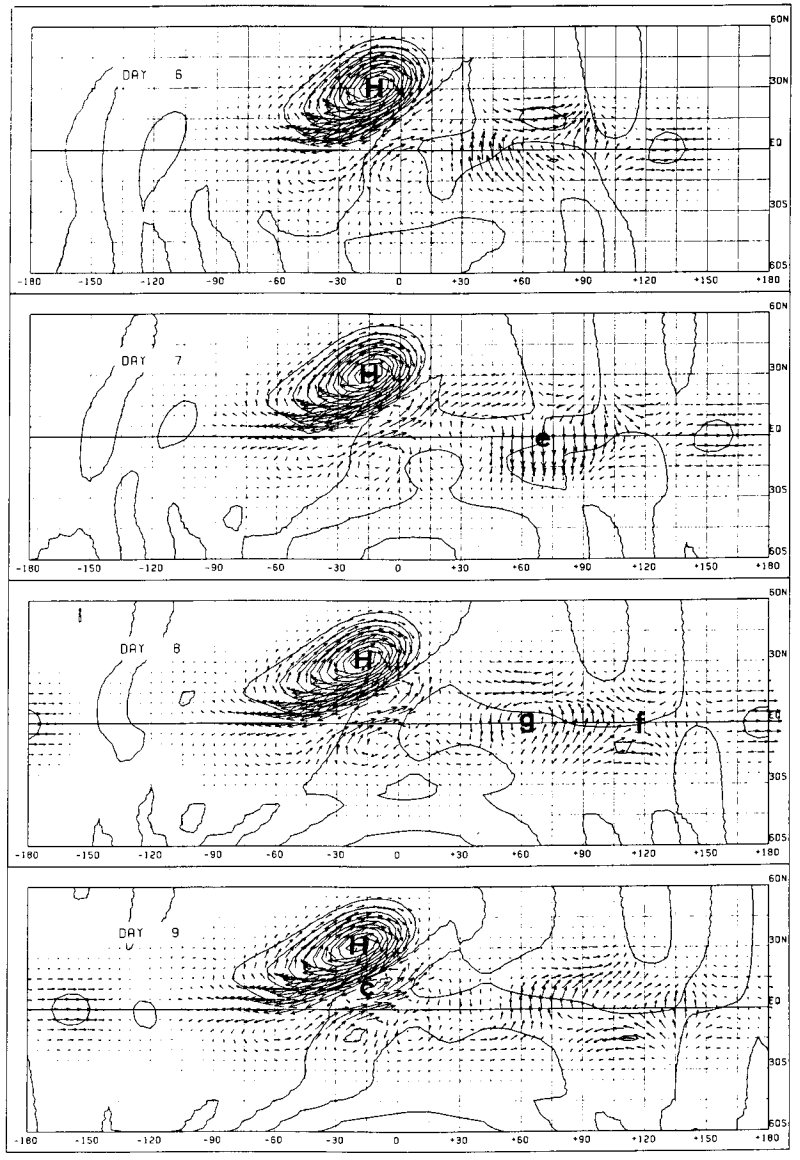
On day 1, after the forcing is switched on, a belt of strong northerly and northeasterly wind sweeps across the equator. Near the leading edge, the wind blows perpendicular to the isobars away from the high pressure, revealing strong gravity wave characteristics in the initial equatorward propagation of disturbances. More gravity wave characteristics are exhibited on day 2 when a low center and southerly winds appear behind the leading surge winds, which have now penetrated deep into the Southern Hemisphere and are deflected eastwards.
From day 3 onward, the midlatitude anticyclonic circulation around the region of forcing develops a marked northeast- southwest tilt. To its south, a belt of strong northeasterly winds sweeps from the subtropical latitude to the equator. A southwesterly cross-equatorial counter flow around the longitude of the forcing becomes well established after day 6. Sandwiched between the belt of strong northeasterly winds and the southwesterly cross-equatorial flow is an equatorial trough (and shear line) extending south-southwestward from about 15oN to the equator. A cyclonic vortex develops also after day 7 in the Southern Hemisphere, just to the south of the cross-equatorial flow. This large area of complex motions, which constitutes the major response of the tropical atmosphere to the midlatitude forcing, drifts slowly westwards but, for all relevant times, remains near the longitude of the forcing.
The foregoing pattern of response bears a remarkable resemblance to the typical winter season flow pattern (see Fig. 27b in Chapter 1). It suggests strongly that the surge wind belt over the South China Sea and the quasi-permanent equatorial trough north of the Borneo coast are basically features of the dynamical response of the tropical atmosphere to the intense anticyclonic development over China prior to the initiation of a cold surge. This group of responses was identified to be an equatorial Rossby wave group. A computation using only the Rossby wave modes of n = 1 to 9 succeeds in reproducing, as far as a visual examination can tell, exactly all the features described (Fig. 14). This suggests that the high-order latitudinal modes are not important.
|
|
Lim and Chang (1981) gave an explanation also for the evolution of this response in terms of the dispersion behaviour of equatorial Rossby wave groups. From day 3 onward, there is also a group of disturbances that splits off from the Rossby mode response and propagates eastward along the equator. A band of westerlies leads the way at a speed of 30 m s.1. This band of equatorial westerlies is easily identified as a Kelvin wave group. Following behind the Kelvin wave group there are some disturbances with a complicated and rapidly changing pattern. These are due mainly to the juxtaposition of a mixed Rossby-gravity wave group and an n = 0 inertia-gravity wave group. They reveal their identity clearly on day 8, when the equatorial eddy of the mixed Rossby-gravity waves and the col pattern of the n = 0 inertia-gravity waves (Fig. 13g and f respectively) are clearly displayed. Although the phase velocity of mixed Rossby-gravity waves is westward, their group velocity is always eastward, and this accounts for the eastward propagation of the mixed Rossby-gravity wave group. These eastward-propagating disturbances offer a plausible explanation for the drifting cloud clusters observed by Williams (1981) and Lau (1982). It is interesting also to regard this flow evolution as a geostrophic adjustment process on an equatorial β-plane. Motions generated by the pressure pulse gradually separate themselves into a geostrophic component and an ageostrophic component. The geostrophic component here is the Rossby wave group, which has quasi-geostrophic flow even at equatorial latitudes and evolves in time into a pattern resembling the winter flow field of the Southeast Asia region. The ageostrophic component concentrates its energy into the n = -1 mode Kelvin waves and the n = 0 mode mixed Rossby-gravity waves and inertia-gravity waves in the form of a complicated train of eastward-propagating disturbances.
In summary, Lim and Chang (1981) investigated the dynamics of midlatitude tropical interactions based on the concept of vertical modes. When the mean winds and damping effects are independent of the vertical coordinates, when there is no planetary boundary layer effects, and when the stability parameter is a function of the vertical coordinate only, the equations of motion may be separated into a complete set of vertical modes. Each of these modes is characterized by an equivalent depth, and the evolution of its horizontal structure is governed by a shallow-water equation system having the equivalent depth as its scale height.
It turns out that the existence of horizontal wind shear does not affect the separation of motions into vertical modes, but can lead to qualitative changes in the horizontal structure of the vertical modes. Vertical modes of large equivalent depth (c > 120 m s-1) have a nearly constant profile in the troposphere. They represent atmospheric motions that have a barotropic structure. Vertical modes with a medium equivalent depth (30 m s-1 < c < 50 m s-1) have a single phase reversal in the midtroposphere (and probably more phase reversals in the stratosphere). Motions associated with these modes have opposite phase in the upper and the lower troposphere, i.e. they are baroclinic motions. In an equatorial β-plane model, free waves of the large equivalent-depth modes have broad latitudinal extent. Motions associated with these modes readily propagate to high latitudes and tend to spread their energy over the whole globe. Tropical influences spread to high latitudes from the tropics, such as the teleconnection patterns, therefore have barotropic vertical structure. Free waves of the medium equivalent-depth modes are trapped within the tropics. Motions associated with these modes excited in the midlatitudes tend to propagate equatorward and hence bring midlatitude influence to the tropics. Tropical motions forced from midlatitudes therefore have baroclinic structure.
When damping is weak, the small equivalent-depth modes (c < 20 m s-1) may survive their slow meridional propagation and exhibit themselves in equatorial motions of complicated vertical structure (short vertical wavelength).
The mechanisms of midlatitude influence on the tropics were clearly illustrated by a study of atmospheric response to a midlatitude pressure surge. In the midlatitudes, the pressure surge generates a simple anticyclonic circulation, which gradually develops northeast-southwest tilt. However, much of the motion excited by the pressure surge spreads equatorward. The energy of the ageostrophic flow components concentrates into equatorial Kelvin waves and mixed Rossby-gravity waves, which are manifest as disturbances propagating eastward along the equator. The energy residing in geostrophically-balanced flow goes into equatorial Rossby waves. The dispersion of equatorial Rossby wave groups gives rise to a complex flow pattern with a band of strong northeasterly winds (the surge), an equatorial trough, and a cross-equatorial current. All these features bear remarkable resemblance to the typical winter flow pattern over Southeast Asia.
A very important basic question that has not been addressed in this chapter is the interaction of heat sources and atmospheric motions. Unlike our models where heat sources are prescribed, heat sources in the real atmosphere are often forced by the motion field. The feedback of motion field to heat source in the tropics is basically the problem of parameterization of cumulus convection a problem where basic understanding is still lacking. Previous theoretical studies addressing this problem are mostly based on the CISK formulation, which is itself based on rather restrictive and somewhat artificial assumptions. To make significant advance in this problem, we will probably need to carry out further studies using numerical models with physically realistic parameterization schemes for convective heating. Although we are still far from a solution of this fundamental problem, the studies that have been carried out should serve to remind us that by using models with prescribed heat sources, we are studying at most half, and probably it is the easier half, of the problem.
to be continued ...7.4 References
Gill, A. E., 1980: Some simple solutions for heat-induced tropical circulations.
Gill, A. E., 1982:
Lim, H., and C.-P. Chang, 1981: A theory of midlatitude forcing of tropical motions during winter monsoons. J. Atmos. Sci., 38, 2377-2392. (click here)
Silva-Dias, P. L., W. H. Schubert, and M. DeMaria, 1983: Large-scale response of the tropical atmosphere to transient convection.
Longuet-Higgins, M. S., 1968: The eigenfunctions of Laplace's tidal equations over a sphere.
Webster, P. J., 1972: Response of the tropical atmosphere to local steady, forcing.
7.5 Other references
Copyright © Roger Smith, Date 11 Jun 2015