Lectures on Tropical Meteorology
Chapter 6. Waves at low latitudes
A characteristic of the atmosphere is its shallow depth; 99% of the mass lies below a height of 30 km whereas the mean earth radius is 6,380 km. Over this 30 km which extends into the middle stratosphere there is a considerable variation in the vertical structure. However much can be learned about low latitude motions by considering the atmosphere to be a uniform layer of fluid with variable depth. Put another way, consideration of the horizontal structure of the vertical mean atmosphere yields rich information about the predominant wave modes, specially at low latitudes. The classical papers on this subject are those of Matsuno (1966) and Longuet-Higgins (1968) with important contributions also from Webster (1972) and Gill (1980) amongst others. A recent review is given by Lim and Chang (1987).
Although we begin our study by assuming a uniform vertical structure, we shall find that the effort is not in vain for it turns out that the solutions to the divergent barotropic system are, in fact, the horizontal part of the baroclinic modes.
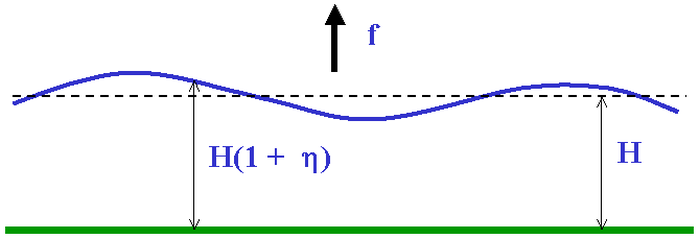
In contrast to Longuet-Higgins (1968) and Webster (1972) who use full-spherical geometry, we follow Matsuno (1966) and Gill (1980) and consider motions on an equatorial beta plane. To begin with, we review the theory of wave motions in a divergent barotropic fluid on an f-plane or on a mid-latitude β-plane as described in DM, Chapter 11. The basic flow configuration is shown in Fig. 1. The fluid layer has undisturbed depth H. [DM refers to my Dynamical Meteorology lectures: (click here)]
|
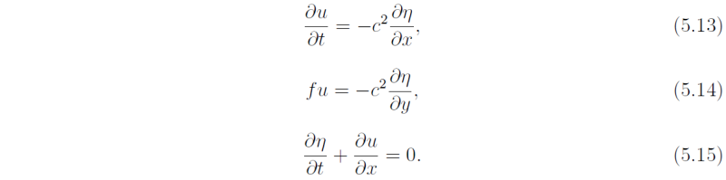
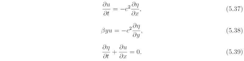
We consider small amplitude perturbations about a state of rest in which the free surface elevation is H(1 + η). As shown in DM, the linearized "shallow-water" equations take the form
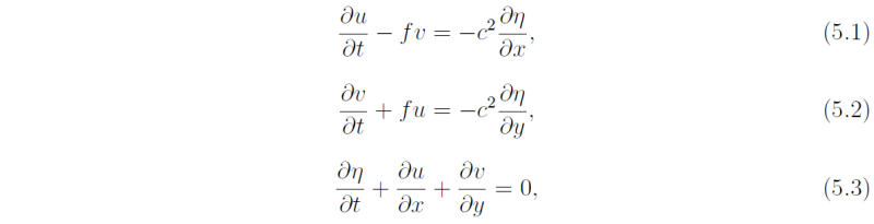
where c = √(gH) is the phase speed of long waves in the absence of rotation (f = 0).
On an f-plane, Eqs. (5.1)-(5.3) have sinusoidal travelling wave solutions in the x-direction with wavelength 2π/k and period 2π/&omega (wavenumber k, frequency &omega) of the form
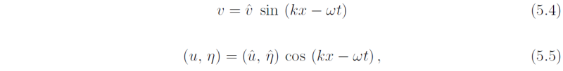
where uhat, vhat and ηhat are constants, provided

This dispersion relation yields &omega = 0, which corresponds with a steady (∂/∂t = 0) geostrophic flow, or ω2 = f2 +c2k2, corresponding with inertia-gravity waves. The phase speed of these waves, cp, is given by

where LR = c/f is the Rossby radius of deformation. Clearly, the importance of inertial effects compared with gravitational effects is characterized by the size of the parameter LR2k2, i.e. by the wavelength of waves compared with the Rossby radius of deformation.
On a mid-latitude β-plane where f is a function of y (specifically, where f = f0 + βy (f0 ≠ 0), it is inconsistent to seek a solution of the form (5.4)-(5.5) with uhat, vhat and ηhat as constants, unless meridional particle displacements are relatively small. In that case, the effects of variable f can be incorporated by replacing the second equation of (5.1)-(5.3) by the vorticity equation

where

Note that variations of f are included only in so much as they appear in the advection of planetary vorticity by the meridional velocity component. Substituting again (5.4) into (5.1), (5.8) and (5.9) shows that, solutions are possible now only if ω satisfies the equation

It is convenient to scale ω by f0 and k by 1/LR, say ω = f0ν, k = m/LR. Then (5.10) reduces to

where LR/f0. At latitude 45o, β/f0 = 1/a, where a is the earths radius. It follows that for Rossby radii LR << a, then ε << 1.
When ε = 0, implying that β = 0, Eq. (5.11) has solutions ν = 0 and ν = μ2 + 1 as before.
If ε << 1, there is a root of 0(ε) which emerges if we set

which in dimensional form, ω = -βk/ [k2 + 1/LR2], is the familiar dispersion
relation for
|
The equation set (5.1)-(5.3) has a solution in which
Cross-differentiating (5.13) and (5.15) to eliminate u gives

which has a general travelling-wave solution of the form

where F and G are arbitrary functions. Define X = x - ct and Y = x + ct. Then using (5.15) we have
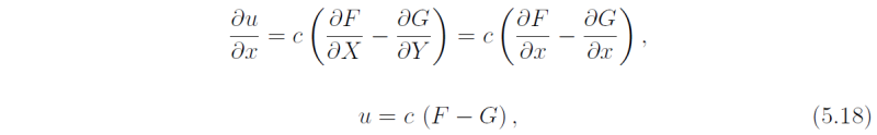
which may be integrated partially with respect to x to give ignoring an arbitrary function of y and t. Substitution of (5.18) in (5.14) gives

and since F and G are arbitrary functions we must have

and

These first order equations in y may be integrated to give the y dependence of F and G, i.e.

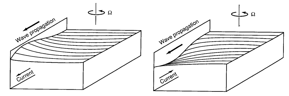
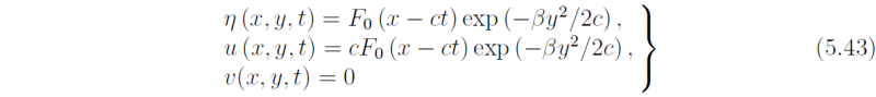
In the configuration shown in Fig. 5.2, we must reject the solution G as this is unbounded as y → ∞. In this case, the solution is

This represents the surface elevation of a wave that moves in the positive x-direction with speed c and decays exponentially away from the boundary with decay scale c/f which is simply the Rossby length, LR. The solution for u from (5.18) is simply

The Kelvin wave is essentially a gravity wave that is "trapped" along the boundary by the rotation. The velocity perturbation u is always such that geostrophic balance occurs in the y direction, expressed by (5.14). If the fluid occupies the region y < 0, then the appropriate solution is the one for which F0 ≡ 0 and then

Again this represents a trapped wave moving at speed c with the boundary on the right in the Northern Hemisphere (when f > 0) and on the left in the Southern Hemisphere (when f < 0).
6.1 The equatorial beta-plane approximation
At the equator, f0 = 0, but β is a maximum. In the vicinity of the equator, (5.1)-(5.3) must be modified by setting f = βy. This constitutes the equatorial beta-plane approximation that may be derived from the equations for motion on a sphere (see e.g. Gill, 1982, sec. 11.4). The perturbation equations are now
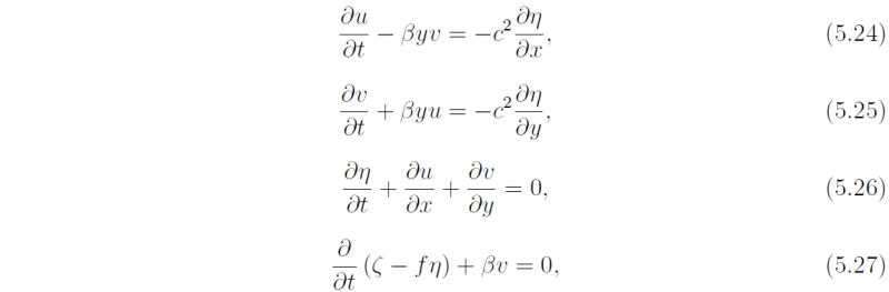
where again

Taking
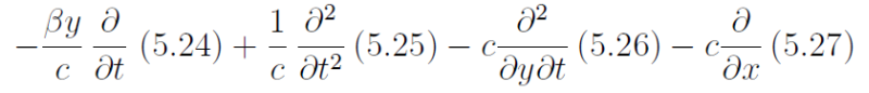
and using (5.28) and remembering that f = βy gives

which has only the dependent variable v. We follow the usual procedure and look for travelling-wave solutions of the form

whereupon vhat(y) has to satisfy the ordinary differential equation obtained by substituting (5.30) into (5.29). Note that, unlike the previous case we cannot assume that vhat is a constant because Eq.(5.29) has a coefficient (namely f2) that depends on y. The equation for vhat(y) is

Before attempting to find solutions to this equation we scale the independent variables t, x, y, using the time scale (2βc)-1/2 and length scale (c/2β)-1/2, the latter defining the equatorial Rossby radius LE. This scaling necessitates scaling ω = (2βc)-1/2ν and k = (c/2β)-1/2μ also. Then the equation becomes

which is the same form as Schr&umo;dingers equation that arises in the theory of quantum mechanics. The solutions are discussed succinctly by Sneddon (1961, see especially Chapter V). A brief sketch of the main results that we require are given in an appendix to this chapter. There it is shown that solutions for vhat that are bounded as |y| → ∞ are possible only if

These solutions have the form of parabolic cylinder functions. In dimensional terms,

which on multiplication by 2-n/2 can be written as

where Dn is the parabolic cylinder function of order n and Hn is the Hermite polynomial of order n. In dimensional form the corresponding dispersion relation, (5.33), is

Like (5.10), this is a cubic equation for ω for each value of n and evidently a whole
range of wave modes is possible. We shall consider the structure of these presently.
6.2 The Kelvin wave
First we note that (5.32) has a trivial solution vhat = 0. As in the case of the Kelvin wave discussed earlier, this solution corresponds with a nontrivial wave mode. To see this we substitute vhat = 0 into Eqs. (5.24)-(5.26) to obtain
These equations are identical with (4.12) if we set f = βy in (5.14). In particular the solutions for η and u are exactly the same as (5.17) and (5.18), respectively. Then (5.38) gives

and

analogous to (5.19) and (5.20). Now (5.40) has the solution

whereas the solution for G is unbounded as y → ± ∞. Therefore Eqs. (5.37)-(5.39) have a solution
This solution is called an equatorial Kelvin wave. It is an eastward propagating gravity wave
that is trapped in the equatorial wave guide by Coriolis forces. Note that it is nondispersive
and has a meridional scale on the order of LE = (c/2β)-1/2.
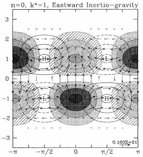
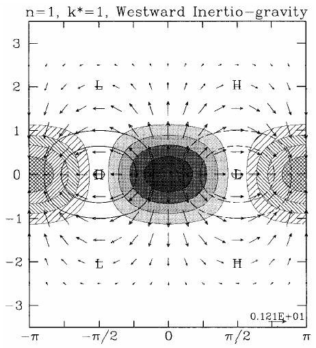
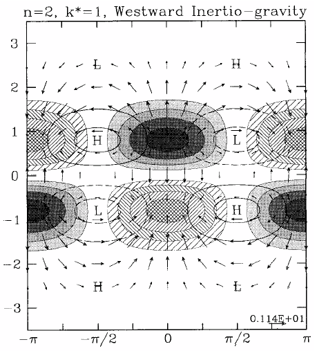
6.3 Equatorial gravity waves
We return now to the dispersion relation (5.36). For n ≥ 1, the waves subdivide into two classes like the solutions of (5.10). There are two solutions for which βk/ω is small, whereupon the dispersion curves are given approximately by

The form is similar to that for inertia-gravity waves (sometimes called Poincaré
waves also - e.g., in Gill, 1982). These waves are equatorially-trapped gravity waves,
or equatorially-trapped Poincaré waves.
6.4 Equatorial Rossby waves
There are solutions also of (5.36) for which ω2/c2 is small. Then the dispersion relation is approximately

These modes are called equatorially-trapped planetary waves or equatorially trapped
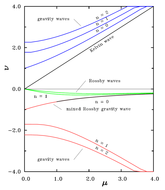
Rossby waves. The various dispersion curves are plotted in Fig. 5.3. This figure
includes also the dispersion curves for the case n = 0 described below and for the
Kelvin wave.
6.5 The mixed Rossby-gravity wave
When n = 0, Eq. (5.33) may be written

The solution ν = -μ must be excluded since it leads to an indeterminate solution for u (see later). Therefore the solutions are, in dimensional form,

and

which represents an inertia-gravity wave if k is small and a Rossby wave if k is large
(see Ex. 5.2). Note that as k → 0, ω- ≈ -(cβ)1/2,
which agrees with the long wavelength limit of the inertia-gravity wave solution (5.44), while
as k → ∞, ω- ≈ -β/k, which agrees with the limit of
the Rossby wave solution (5.45). Therefore, the solution n = 0 is called a
To calculate the complete structure of the various wave modes we need to obtain
solutions for u and η corresponding to the solution for v in Eq. (5.34).
We return to the linearized equations (5.24)-(5.28). The substitution

in (5.24) and (5.26) gives
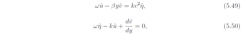
which may be solved for uhat and ηhat in terms of vhat and dvhat/dy, i.e.,
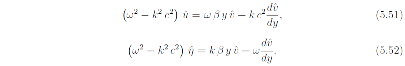
With the previously introduced scaling and y = LEY , these become

and

Also, from (5.34)

whereupon

We use now two well-known properties of the Hermite polynomials:

and

It follows that

and

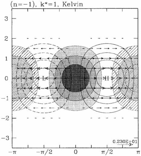
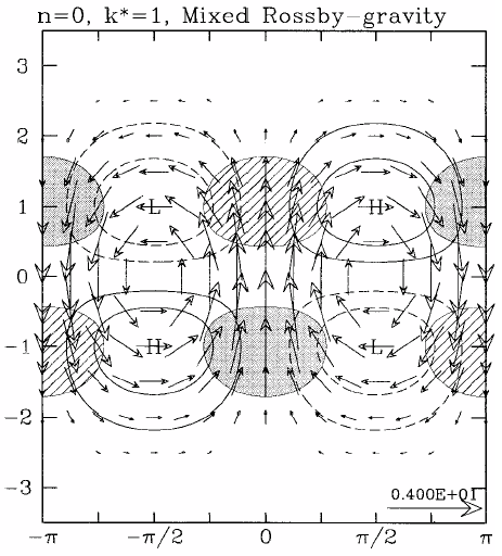
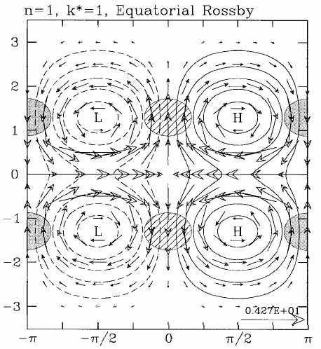
Figure 4 shows the horizontal structure of the Kelvin wave and of a westward propagating mixed Rossby-gravity wave. Air parcels move parallel to the equator in the case of the Kelvin wave and move clockwise around elliptical orbits in the case of the mixed wave. Plots for other equatorial wave modes are shown in Figs. 5 and 6.
|
|
|
6.6 The equatorial waveguide
The equatorial wave-guide equation (5.31) has the form

where

using (5.36). Solutions thereto have a wave-like structure in the meridional (y-) direction if y < yc and an exponential structure if y > yc. Thus yc corresponds with a critical latitude for a particular mode, a latitude beyond which wave-like propagation is not possible. If the phase of a particular wave changes rapidly enough with y, we can define a local meridional wavenumber κ for each value of y, the assumption being that κ varies only slowly with y. One may then use the WKB technique outlined in Gill (1982, sec. 8.12, pp 297-302) to find approximate solutions to (5.61). Such solutions have the form

where

This approximate solution is valid provided that

At the equator δ = 1/[2(2n + 1)2] i.e. the approximate solution is valid provided n is large. The group velocity of waves follows from (5.62), i.e.,

whereupon wave packets propagate along rays dxdt = cg , or in this case,

Using (5.64) it follows readily that ray paths have the form

i.e., they are sinusoidal paths about the equator in which wave energy is reflected at the critical latitudes y = ±yc.
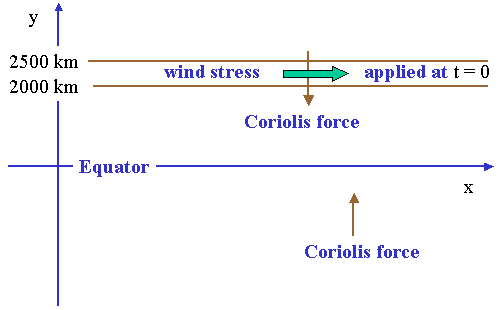
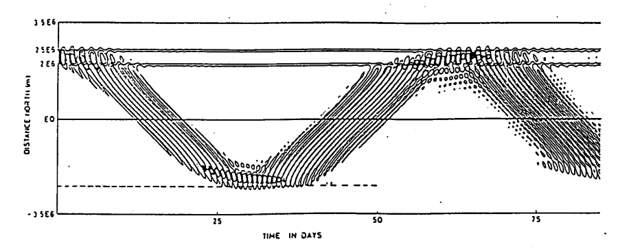
A simple thought experiment exibiting this kind of behaviour is the response of a resting ocean to the sudden application of a uniform wind stress over a small range of latitudes that are remote from the equator (Fig. 7).
|
The wind stress results in the generation of inertial waves with no variation in x, i.e. k = 0. Then the term β/ω can be ignored in (5.66) and (5.68). The path followed by these waves can be calculated from dy/dt = cgy. Since k = 0 the group velocity is given by

Integration of (5.69) with respect to time indicates that the path followed by the waves is sinusoidal in time about the equator as shown in Fig. 8.
|
Another effect of the waveguide is the discretization of modes n = 1, 2, .... in the meridional direction. For long inertia-gravity waves (k → 0) this implies a discrete set of frequencies given by

obtained from (5.62). Gill (1982, p 442) notes that this frequency selection shows up in Pacicfic sea-level records because variations associated with the baroclinic mode have magnitudes of the order of centimeters which is large enough to be detected. For these modes c ≈ 2.8 m s-1 giving periods of 5½, 4 and 3 days for n = 1, 2 and 3, respectively. See Gill (1982, p442) for further details.
6.7 The planetary wave motions
Planetary waves have the approximate dispersion relation (5.45) which, in the long-wave limit (k → 0), is ω ≈ kc/2n +1). The phase speed ω/k is in the opposite direction to the Kelvin wave (i.e. westward) and the amplitudes are reduced by factors 3, 5, 7 etc. For example, for the first baroclinic mode in the Pacific Ocean, c = 2.8 m s-1, so that the planetary wave with n = 1 has speed 0.9 m s-1. This mode would require 6 months to cross the Pacific Ocean from east to west. Other modes would be slower. These facts have implications for the coupled atmospheric-ocean response to perturbations in the tropics.
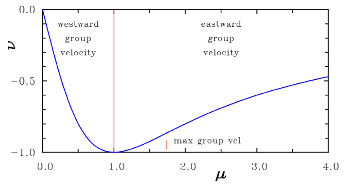
Figure 9 shows the dispersion curve (5.45) for the planetary wave modes.
|
Differentiating (5.45) with respect to k gives

Thus the curve has zero slope where dω/dk = 0, i.e.

where fc = βyc, and yc is defined by (5.62).
At the point k = k* the frequency has a

For example when n = 1, this corresponds to a minimum period of 31 days for a first baroclinic ocean mode with c = 2.8 m s-1, 74 days for a higher mode with c = 0.5 m s-1, and 12 days for an atmospheric mode with c = 20 m s-1.
For waves with wavelength shorter than 2π/k, the group velocity (∂ω/∂k) is positive (i.e. eastward) and therefore in the direction opposite to the phase velocity. The maximum group velocity is cg = ⅛c/(2n + 1) when k = [3(2n + 1)/LE2]½. Thus only short waves can carry information eastwards and then at only one eighth of the speed at which long waves can carry information westwards.
6.8 Baroclinic motions in low latitudes
The equations for small amplitude perturbations to an incompressible stratified (Boussinesq) fluid at rest are
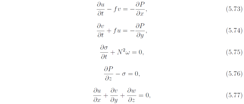
where P = p/pbar. Elimination of w and σ from (5.75) - (5.77) gives

If we choose P to satisfy the equation (5.79)

then (5.79) becomes

whereupon Eqs. (5.73), (5.74) and (5.80) have exactly the same form as the shallow water equations (5.1) - (5.3) if we identify c2η in the latter with P in the former. Equation (5.79) with appropriate boundary conditions leads to an eigenvalue problem for the vertical structure of wave perturbations and the corresponding eigenvalue c. Consider the case of an isothermal atmosphere with N2 = constant. Then differentiating (5.79) with respect to z and t and using (5.75) and (5.76) to eliminate P in preference to w gives

For a liquid layer bounded by rigid horizontal boundaries at z = 0 and z = H, where w = 0, Eq. (5.81) has the solution

and the corresponding eigenvalues are
As usual, the gravest mode (the one with the largest phase speed, the case n = 1) has a single vertical velocity maximum in the middle of the layer, z = ½H. Taking typical values for N (= 10-2 s-1) and H (the tropical tropopause = 16 km), the phase speed of the gravest mode c1 = 51 m s-1.
It is easily verified that (5.81) holds even if N is a function of z, but then the eigenvalue problem will be more difficult to solve.
6.9 Vertically-propagating wave motions
In an unbounded vertical domain and when N is a constant, Eq. (5.81) has solutions proportional to exp(±imz), where m2 = N2/c2. Therefore, the system of equations (5.73) - (5.77) have solutions in which, for example,

where

Note that c is a property of the mode in question and is equal to the phase speed only in special cases such as the Kelvin wave. For an isothermal compressible atmosphere, Eq. (5.81) is a little more complicated, but is still given by (5.84) to a good approximation provided that 1/(4m2Hs2 << 1, where Hs is the scale height. Even for vertical wavelength of 20 km, this number is only about 0.03, so that the incompressible approximation is reasonable.
Now consider the dispersion relation ω = ω(k) for the various types of waves with vector wavenumber k = (k,m). It is convenient to scale the wavenumber components by writing k = (β/ω)k* and m = (βN/ω2)m*. Then, the dispersion relation for the Kelvin wave, ω = kc becomes

For the mixed Rossby- gravity wave (n = 0), ωm/N - k - β/ω = 0 from (5.46], which becomes,

The remaining waves satisfy (5.36)


or

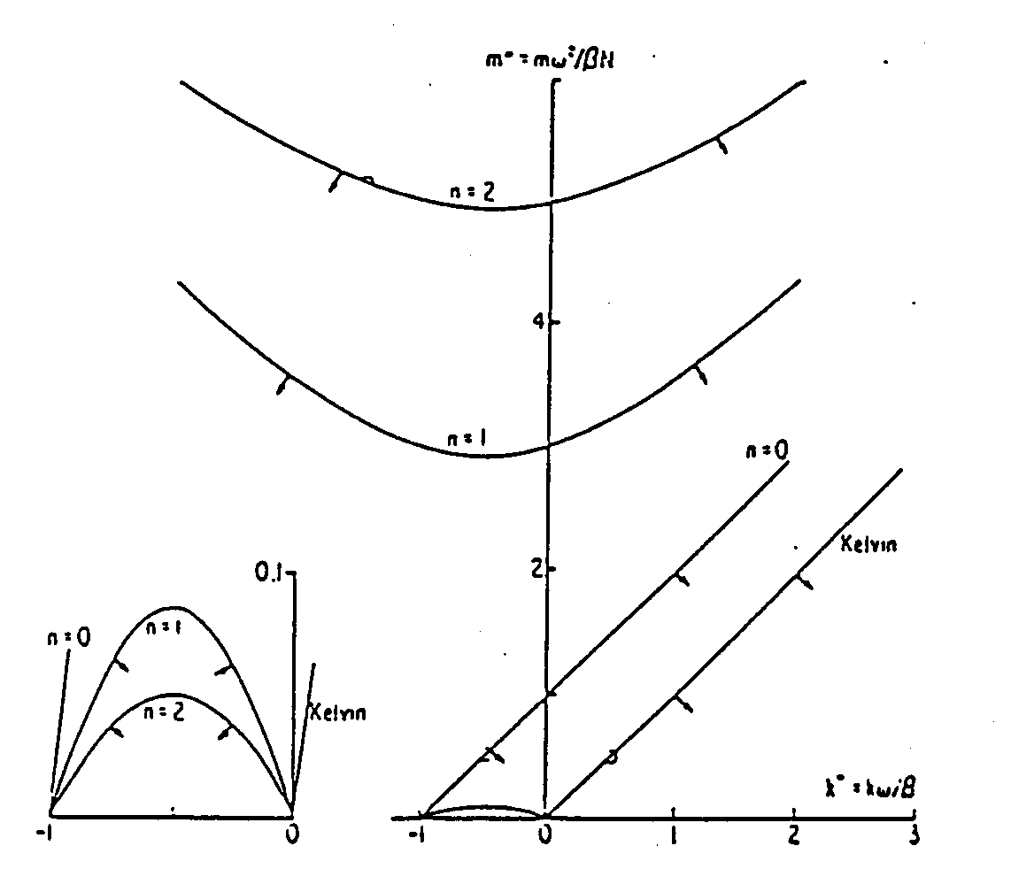
It can be shown that modes corresponding with the positive root in (5.87) are gravity waves while those corresponding with the negative root are planetary waves. The full set of dispersion curves is shown in Fig. 10. The gravity wave curves are the hyperbolae in the upper part of the diagram. The planetary wave curves are hyperbolae also and are shown on the expanded plot in the inset. The corresponding curves in the k-plane are the curves of constant frequency. The group velocity cg = ∇kω is at right angles to these curves and in the direction of increasing ω. The corresponding directions are shown in Fig. 10.
|
We carry out the calculations for the Kelvin wave and mixed Rossby-gravity waves.
6.9.1 Kelvin wave
In this case

Then

whereupon

Note that cg3 > 0 if m < 0, i.e. the Kelvin wave solution that propagates energy vertically upwards has phase lines that slope upward in the eastward
direction. Figure 11 shows the structure of this mode.
In this case ω satisfies whereupon i.e. Now (5.88) gives from which it follows that the mixed Rossby-gravity wave, i.e. the solution for the negative square root, has ω < 0. From (5.89) we see that this
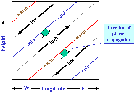
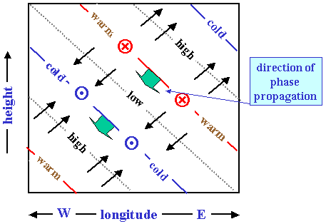
has an upward-directed group velocity if m > 0. Thus the phase lines of the mixed Rossby-gravity wave tilt westward with height (Fig. 12). Figure 5.12
shows the structure of this mode also. Note that poleward-moving air is correlated with positive temperature perturbations so that the eddy heat flux v'T' '
averaged over a wave is positive. The mixed Rossby-gravity wave removes heat from the equatorial region. Both Kelvin wave and mixed Rossby-gravity wave modes have been identified in observational data from the equatorial stratosphere. The observed Kelvin
waves have periods in the range 12-20 days and appear to be primarily of zonal wavenumber 1. The corresponding observed phase speeds of these waves relative
to the ground are on the order of 30 m s-1. In applying our theoretical formulas for the meridional and vertical scales, however, we must use
the Doppler-shifted phase speed cp - U, where U is the mean zonal wind speed. Assuming U = -10 m s-1, cp - U =
40 m s-1, whereupon LE = √[(cp - U)/β] ≈ 1300km. This corroborates with observational evidence that
the Kelvin waves have significant amplitude only within about 20o latitude of the equator. Knowledge of the observed phase speed also allows one
to calculate the theoretical vertical wavelength of the Kelvin wave. Assuming that N = 2 × 10⁻² s-1 (a stratospheric value)
we find that
which agrees with the vertical wavelength deduced from observations. (Note that for the Kelvin wave, cp = c).
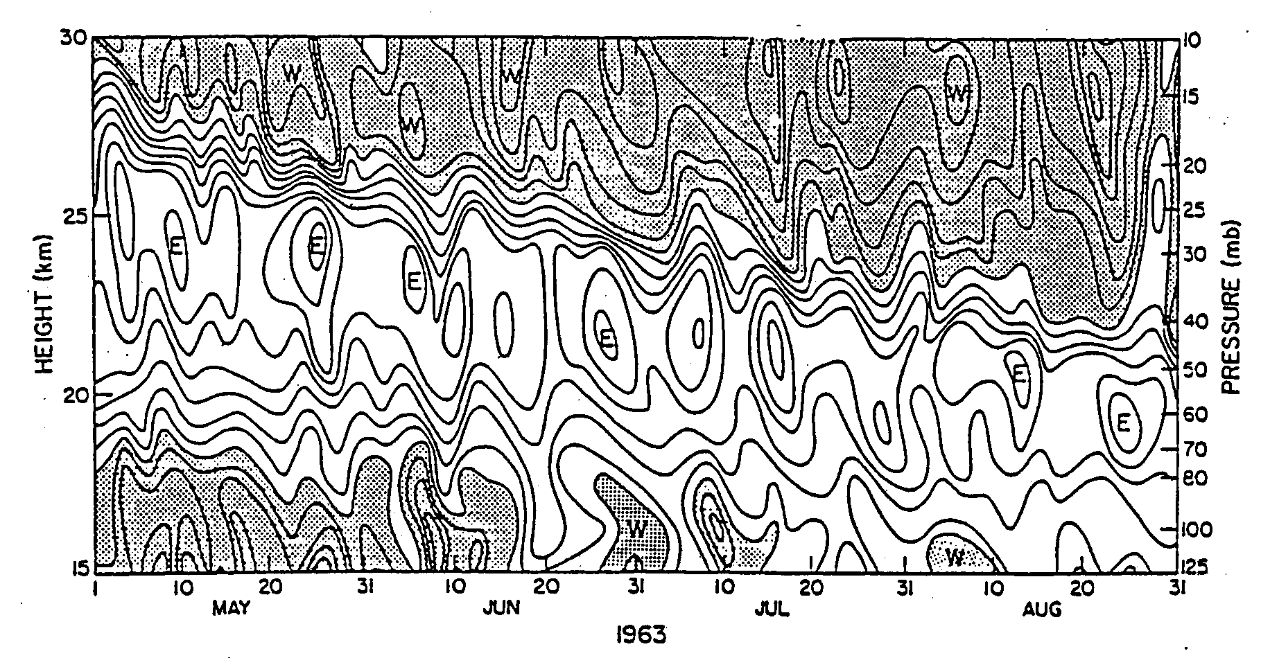
Figure 13 shows an example of zonal wind oscillations associated with the passage of Kelvin waves at a station near the equator. During the
observational period shown in the westerly phase of the so-called quasi-biennial oscillation is descending so that at each level there is a general
increase of the mean zonal wind with time. Superposed on this trend is a large fluctuating component with a period between speed maxima of about 12
days and a vertical wavelength (computed from the tilt of the oscillations with height) of about 10-12 km. Observations of the temperature
field for the same period reveal that the temperature oscillation leads the zonal wind oscillation by one quarter of a cycle (that is, the maximum
temperature occurs one quarter of a period prior to maximum westerlies), which is just the phase relationship required for Kelvin waves (see Fig. 11).
Furthermore, additional observations from other stations indicate that these oscillations do propagate eastward at about 30 m s-1. Therefore
there can be little doubt that the observed oscillations are Kelvin waves. The existence of the mixed Rossby-gravity mode has been confirmed also in observational data from the equatorial Pacific. This mode is most easily
identified in the meridional wind component, since v is a maximum for it at the equator. The observed waves of this mode have periods in the range of
4-5 days and propagate westwards at about 20 m s-1. The horizontal wavelength appears to be about 10,000 km, corresponding to zonal
wavenumber-4. The observed vertical wavelength is about 6 km, which agrees with the theoretically derived wavelength within the uncertainties of the
observations. These waves appear to have significant amplitudes only within about 20o latitude of the equator also, which is consistent
with the e-folding width √[2LE] = 2300 km. Note that in this case, c = cp, but using (5.88) and (5.84), for the
mixed Rossby-gravity wave mode. At present it appears that both the Kelvin waves and the mixed Rossby-gravity waves are excited by oscillations in
the large-scale convective heating pattern in the equatorial troposphere. Although these waves do not contain much energy compared with typical
tropospheric disturbances, they are the predominant disturbances of the equatorial stratosphere. Through their vertical energy and momentum transport
they play a crucial role in the general circulation of the stratosphere. The theory of equatorial waves and their relevance to tropical weather forecasting and climate continues to be a lively topic of research. Below
are a few papers that you may fins of special interest. A recent review is that of Kiladis et al. (2008). Lander, M. A., 1990: Evolution of cloud pattern during the formation of tropical cyclone twins symmetrical with respect to the equator.
Wheeler, M. and G. N. Kiladis, 1999: Convectively coupled equatorial waves: Analysis of clouds and temperature in the wavenumber domain.
Wheeler, M., G. N. Kiladis and P. J. Webster, 2000: Large-scale dynamical fields associated with convectively coupled equatorial waves.
Wheeler, M. and K. M. Weickmann, 2001: Real-time monitoring and prediction of modes of coherent synoptic to intraseasonal tropical variability.
Yang, G-Y, B. Hoskins, and J. Slingo, 2003: Convectively coupled equatorial waves: a new methodology for identifying wave structures in observational data.
Kiladis, G. N., M. C. Wheeler, P. T. Haertel, and K. H. Straub, 2008: Convectively coupled equatorial waves. Yang, G-Y, and B. Hoskins, 2013: ENSO impact on Kelvin waves and associated tropical convection. Copyright © Roger Smith, Date 11 Jun 2015
6.9.2 Mixed Rossby-gravity wave


6.10 Further reading on equatorial waves
6.11 Other references