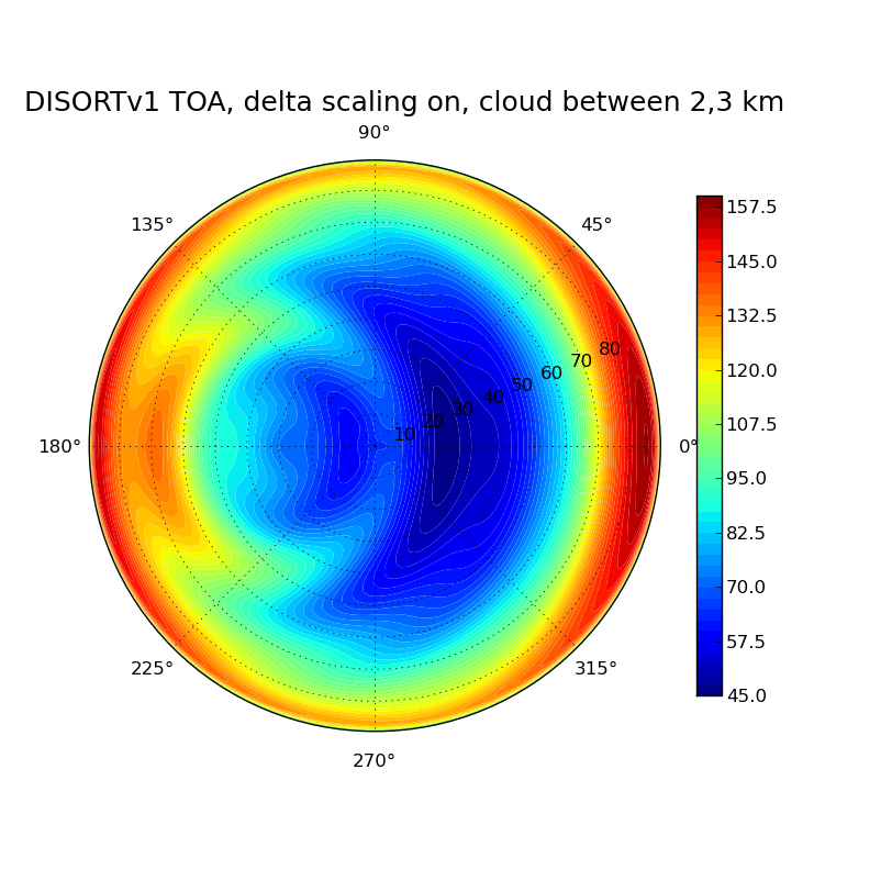
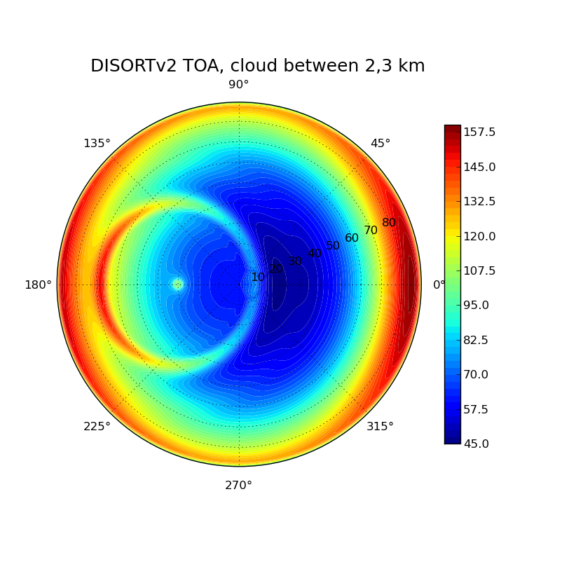
Calculate the radiance field for a cloudy atmosphere at the top of the atmosphere using the DISORT solver. Perform the calculation first for a pure Rayleigh atmosphere (only molecular absorption and scattering) and then include a cloud layer. What changes when you include the cloud? Use version 1 of disort with and without delta scaling (rte_solver disort including exactly the solution method derived in the lecture) and version 2 (rte_solver disort2) which includes a second order intensity correction method. Explain the results in general and the differences between the two solvers.

Use the libRadtran input file and the plotting script from exercise 6 to start.

A cloud layer is included by adding the following lines to the input file

disort1.inp

wc_file 1d                 wc.dat
wc_properties              mie interpolate

More options to specify clouds are available in libRadtran, please check options starting with wc_ (water cloud) and ic_ (ice cloud) in the libRadtran user manual.

In order to use the cloud phase functions using Mie theory you have to copy some data into your libRadtran data directory

 cp /home/data/daten/public/rt-data/optprop_data/wc_new/wc.???.mie.cdf /local/libRadtran-1.5-beta/data/wc

If you do not have the permissions please let me know.

The file wc.dat includes two columns to specify the liquid water content and the effective droplet size:

wc.dat

# z [km]   LWC [g/m^3]  Reff[micrometer]
   3         0           0
   2       0.01         10

This file for example specifies a cloud layer between 2 and 3 km with a liquid water content of 0.01 and an effective droplet radius of 10 μm.

Tips:

In order to generate a line with umus from 0.01 to 1, you may use gawk:

 gawk '{for (i = 1; i<=100; i++)  printf("%g ", 0.01*i)} ' dummy

where dummy is a file including one arbitrary line.

In the plotting script (radfield_polar.py), the plot command should look as follows:

 contourf(phi*pi/180, arccos(umu)*180/pi, rad, N, cmap=cm.jet)

(theta should be in the range from 0° to 90°).

sza 30                   # solar zenith angle
source solar             kurudz_1.0nm.dat
atmosphere_file          us-standard
albedo 0.0               # Surface albedo
nstr                     16
wavelength               500
zout                     toa # defines viewing location at toa
 
#following param defines the angles, that we get results for e.g. the azumithally:
phi 0 2 4 6 8 10 12 14 16 18 20 22 24 26 28 30 ... 360
# and to look down from TOA we have only positive values:
umu 0.01 0.02 0.03 0.04 0.05 0.06 0.07 0.08 ... 1
 
# Note if we'd look up to the sky in case we are at the ground, we take 
# umu -1 -0.99 -0.98 -0.97 -0.96 -0.95 -0.94 ... -0.01
 
 
#In the following we introduce a water vapor file that configures a cloud layer between 2-3 km.
#this is done by the following paramters in libRadtran File:
wc_file 1D                 wc.dat
wc_properties              mie interpolate