
The majority of tropical cyclones develop from pre-existing deep convective cloud systems, essentialy clusters of thunderstorms, in the tropics. However, a few originate from the transformation of existing subtropical weather systems. Only a small fraction of tropical cloud clusters ultimately develop into tropical cyclones. Traditionally, the questions as to how tropical cyclones actually form (the genesis problem) and how they intensify (the intensification problem) have been treated separately. This may be due, in part, to the fact that the early theories for tropical cyclone behaviour were underpinned by axisymmetric models, which were recognized to be inappropriate during the formative stages of storms.
There is accumulating evidence now to suggest that the physical processes involved in tropical cyclogenesis and intensification are the same, but that these processes are intrinsically three-dimensional (Montgomery and Smith 2011, Kilroy et al., 2017, Smith and Montgomery 2023, Chapter 10). Even so, axisymmetric models do provide a useful basis for understanding many aspects of tropical cyclone evolution
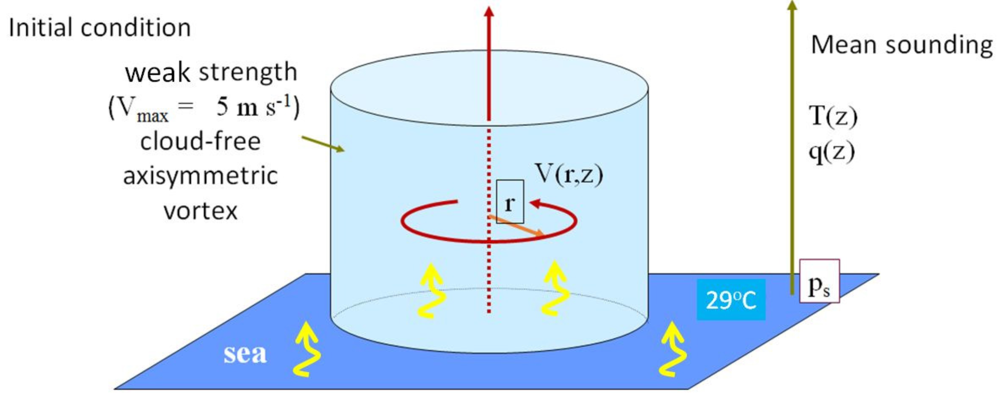
As a pathway towards developing such understanding, many studies have focussed on the so-called prototype problem for intensification. This problem asks: how does a prescribed, initially cloud-free, axisymmetric vortex in a quiescent environment evolve when located over a warm ocean on an \(f\)-plane? Evaporation of sea water at the warm ocean surface serves to maintain deep convective activity as the tropical cyclone develops. The basic flow configuration is shown in Figure 1.
|
An \(f\)-plane is a Cartesian coordinate system in which the vertical axis is normal to the Earth's surface at a given location, the vertical component of the Earth's rotation is treated as a constant and the horizontal components are ignored. The quantity \(f\) equals twice the local rotation rate of the Earth and is called the Coriolis parameter.
The assumption of a quiescent environment has served historically as a simplification for isolating basic aspects of cyclone intensification that do not involve strong interactions with the storm environment. Recent observations and theory pointing to the necessity of a "pouch"-like circulation in the genesis and intensification of these storms provides additional justification for this approach when interpreted in the reference frame moving with the pouch.
Historically, four prominent paradigms have been proposed for understanding tropical cyclone intensification. These were reviewed in a paper by Montgomery and Smith (2014) and include:
the Conditional Instability of the Second Kind (or CISK-) paradigm;
the cooperative intensification paradigm;
a thermodynamic air-sea interaction instability paradigm (widely known as WISHE, an acronym for Wind Induced Surface Heat Exchange); and
the rotating-convection paradigm.
The first three paradigms assume the flow to be axisymmetric, including any explicitly-resolved deep convection. This assumption can be justified as a reasonable approximation to the inner core of well-developed mature storms with an approximately circular eyewall, but is less appropriate for the outer part of such storms, or for storms in their early stages, where observations show that significant flow asymmetries are the norm. In contrast, the rotating-convection paradigm does not assume the flow to be axisymmetric. We focus here on two of these paradigms: the cooperative intensification paradigm, or classical paradigm, and the rotating-convection paradigm. Before describing these paradigms, we review some basic dynamical aspects of vortex development, in general.
|
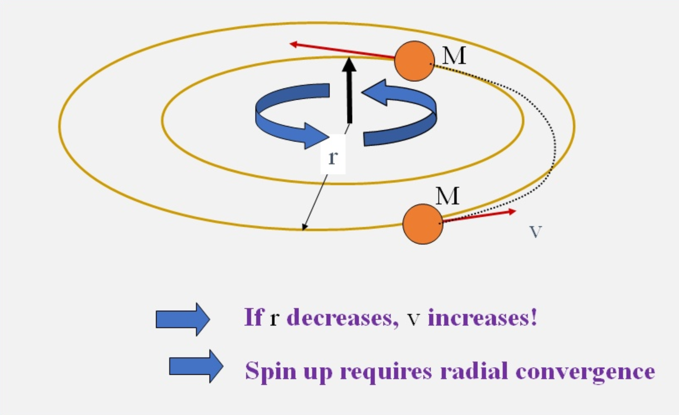
A cornerstone for understanding the spin up of an axisymmetric vortex is the material conservation of the absolute angular momentum, \(M\), above the frictional boundary layer. Material conservation refers to invariance following a moving air parcel. The quantity \(M\) is defined in terms of the tangential velocity, \(v\), the radius from the rotation axis, \(r\), and the Coriolis parameter \(f\), by the relationship $$M = rv + \frac12 fr^2,\quad\textrm{ whereupon }\quad v = \frac{M}{r} - \frac12 fr.$$
Referring to an air parcel moving in an inward-spiralling path where there is no frictional stress in the tangential direction, the material conservation of \(M\) for that parcel implies that the tangential wind speed will increase (Figure 2). Conversely, if the parcel were spiralling outwards, the tangential wind speed will decrease, possibly changing sign if the radial displacement is large enough. We may conclude that spin up of the tangential wind requires radial inflow and that radial outflow leads to spin down. The material conservation of \(M\) follows directly from the tangential momentum equation when there are no frictional or sub-grid-scale forces in the azimuthal direction (see Smith and Montgomery 2023, Section 5.6).
Illustrations of how the foregoing angular momentum principle can be used to understand vortex spin up or spin down is provided by two simple laboratory experiments (Figures 3 and 4).
In general,
|
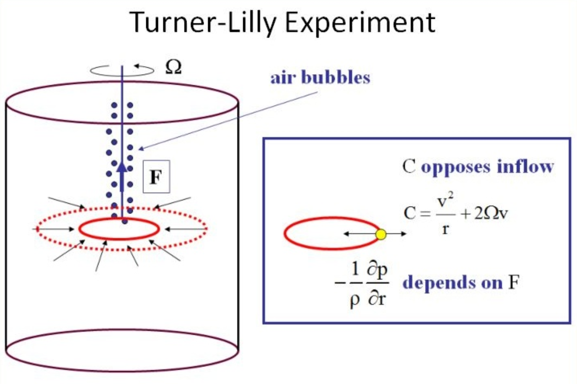
Except in a shallow boundary layer near the lower boundary, converging rings of water conserve their absolute angular momentum and consequently spin faster as they are drawn inwards toward the axis of rotation. The ultimate degree of amplification of the angular velocity depends on how far the rings can be drawn inwards by the overturning circulation produced by the rising bubbles. This inward displacement increases with the bubbling rate, but decreases with increasing background rotation rate. If the forcing is sufficiently large for a given rotation rate, rings of water may be drawn in to relatively small radii before the sum \(C\) of the centrifugal force per unit mass $$ CE = \frac{v^2}{r}, $$
and Coriolis force per unit mass $$ CO = 2\Omega v, $$
opposing the inward motion balance the radial pressure gradient force per unit mass $$ PGF = -\frac{1}{\rho}\frac{\partial p}{\partial r}, $$
induced by the bubbles. It is this pressure gradient force that drives the rings of water inwards (right panel of Figure 3). Again, \(v\) is the azimuthal velocity component and \(r\) is the radius from the rotation axis. In addition, \(f\), now equal to \(2\Omega\), is twice the background rotation rate of the cylinder, \(p\) is the pressure and \(\rho\) is the density of water.
If the forcing is comparatively weak, or if the rotation rate is sufficiently strong, a balance of the radial forces may be achieved before the radial displacement of a water parcel is very large, so that a significant amplification of the background rotation will not be achieved. Clearly, if there is no background rotation, there will be no amplification, and if the background rotation is very weak, the centrifugal and/or Coriolis forces never become large enough to balance the radial pressure gradient, except possibly at large radii from the source of bubbles.
The foregoing arguments emphasize the unbalanced flow adjustment from the instant that the bubbling is turned on, in contrast to the more gradual adjustments that occur typically in tropical cyclones. In fact, the bubbling experiment was originally conceived as one for demonstrating how a tornado vortex might descend from a cloud (Morton, 1966). Nevertheless, if the container is relatively wide and shallow and the bubbles are generated from a ring of tubes, the experiment should be relevant to understanding tropical cyclones also, especially when a vortex has become established at the surface. In particular, as discussed later, the experiment allows one to consider the evolution of the vortex when the bubbling rate is slowly varied, analogous to changes in convective activity in a real storm.
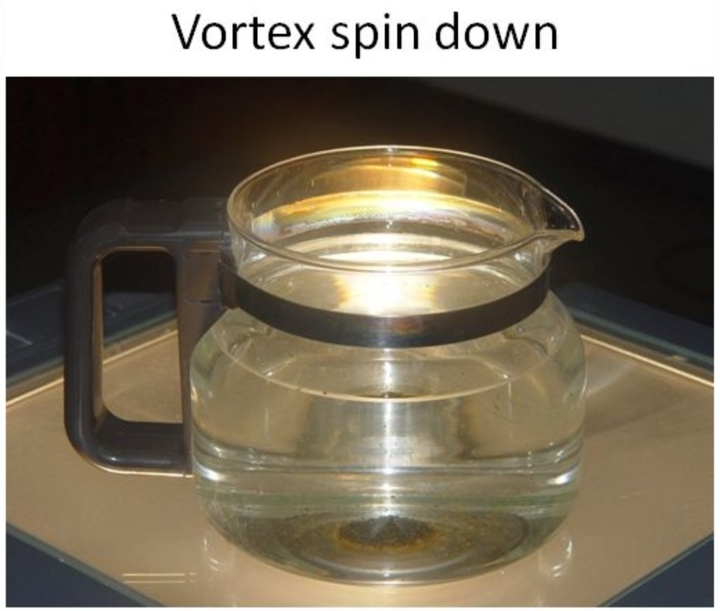
When a concentrated vortex has formed and extended to the lower boundary, frictional effects become important. These may be illustrated by a second experiment that can be easily carried out in the home (Figure 4).
|
The classical spin down problem for a vortex considers the evolution of an axisymmetric vortex above a rigid boundary normal to the axis of rotation. The spin down is primarily a result of the tangential component of generalized Coriolis force, \(-u(v/r + f)\), which depends on the secondary circulation induced by friction above the boundary layer. The direct effect of the frictional diffusion of tangential momentum to the surface with frictional drag at the surface are of secondary importance to the spin down in the parameter regimes relevant to tropical cyclones.
One can demonstrate the frictionally-driven inflow simply by placing tea leaves in a water container and vigorously stirring the water to set it in rotation. After a short time, the tea leaves congregate in a neat pile at the bottom of the container near the axis, as shown in Figure 4. They are swept there by the inflow in the friction layer. Slowly, the rotation in the container declines because the inflow towards the rotation axis in the friction layer has to be accompanied by radially-outward motion in the vortex above this layer in order to satisfy mass continuity.
The depth of the friction layer depends on the viscosity of the water and the rotation rate of the water and is typically only on the order of a millimeter or two in this experiment. Because the water is rotating about the vertical axis, it possesses angular momentum about this axis. Here, because the container, itself, is not rotating, angular momentum is simply the product of the tangential flow speed and the radius.
The classical model for tropical cyclone intensification is built on the seminal studies of the thermally or frictionally-controlled meridional circulation in a circular vortex and of frontal circulations by Eliassen (1951,1962). Similar formulations for the diagnosis and evolution of the balanced tangential and overturning circulation of an idealized axisymmetric tropical cyclone were developed by Willoughby (1979), Shapiro and Willoughby (1982), Schubert and Hack (1982), Schubert and Hack (1983) and Schubert and Alworth (1982).
|
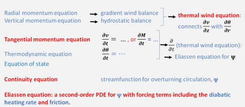
The axisymmetric balance model is based on the momentum equations for the radial, \(u\), vertical, \(w\), and tangential, \(v\), velocity components, a thermodynamic equation for the potential temperature, \(\theta\), or its inverse \(\chi\), an equation of state, and a mass continuity equation for the transverse circulation. The radial and vertical momentum equations are approximated by gradient wind balance and hydrostatic balance, respectively. Elimination of the pressure from these two balance equations gives the
Differentiation of the thermal wind equation partially with respect to time and eliminating the time derivatives using the tangential momentum equation and potential temperature equation gives a diagnostic equation for the transverse, overturning circulation involving \(u\) and \(w\). Finally, using the mass continuity equation to introduce a streamfunction, \(\psi\), for the transverse circulation, one ends up with
The reduced set of balance equations, coloured red in Figure 5, form a prognostic dynamical system that may be solved as follows (Smith et al., 2018):
Given an initial tangential wind profile as a function of \(r\) and \(z\) and a sounding of pressure and temperature at some large radius one can use the thermal wind equation to determine the pressure field (the characteristics of this first-order partial differential equation are just the isobars), the balanced density and potential temperature distribution at the initial time;
Then, given some distribution of diabatic heating and friction, one can solve the Eliassen equation for \(\psi(r,z)\), from which the radial and vertical velocity components can be obtained;
Finally, the tangential momentum equation can be applied to advance the solution in time, and so on.
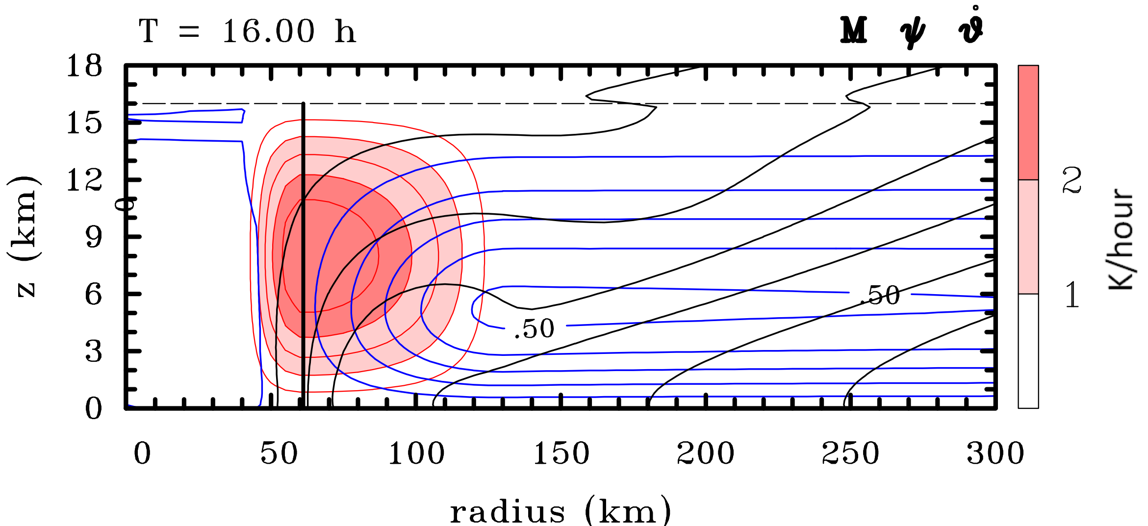
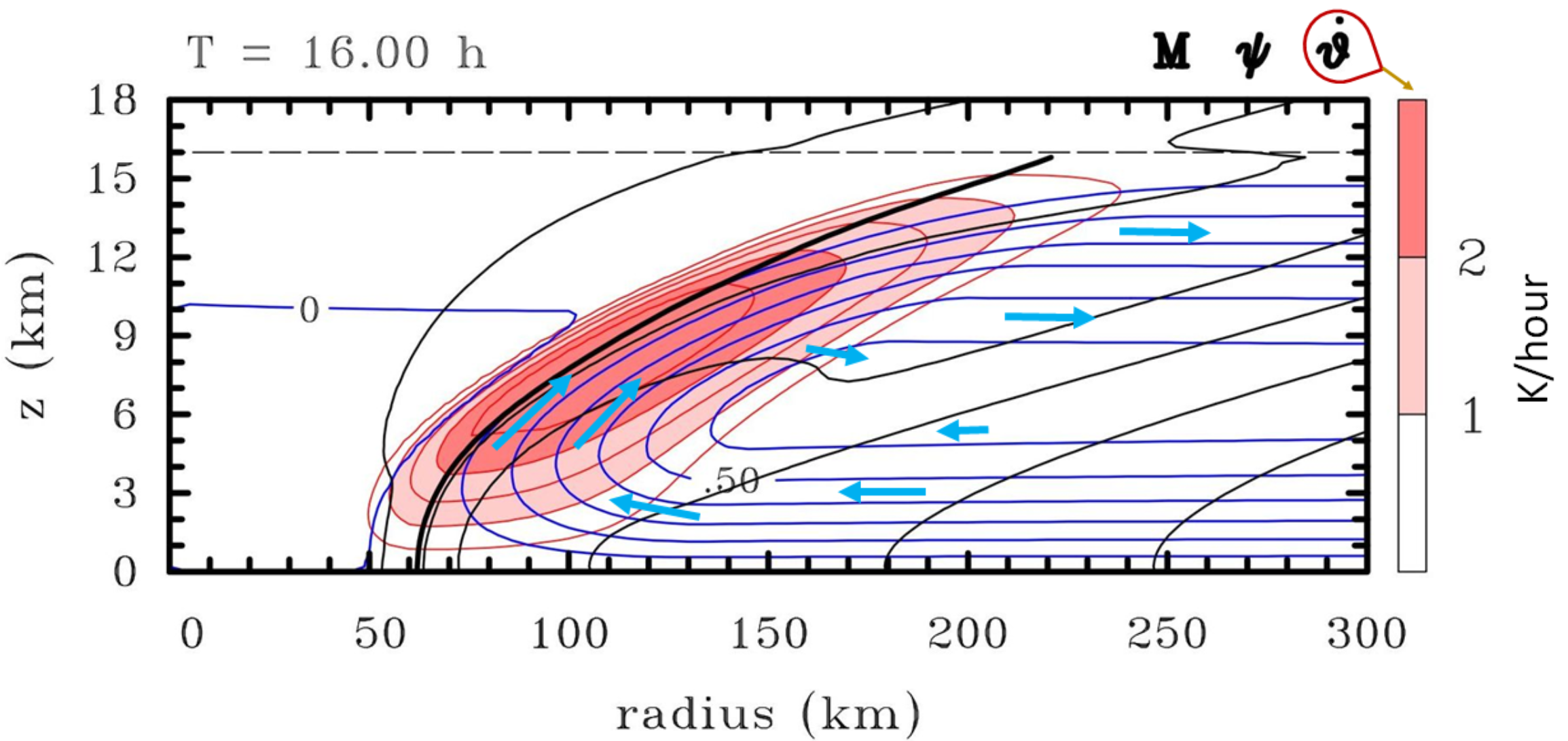
The solution character in two typical prognostic calculations of
|
Note that the streamlines generally cross the \(M\)-surfaces in the lower troposphere in the direction of diminishing \(M\). Thus, invoking the principle of material conservation of absolute angular momentum, \(M\) (Section 3.2), the \(M\)-surfaces will be advected inwards there and the tangential velocity will increase. In the upper troposphere, the \(M\)-surfaces will be advected outwards and the tangential velocity will decrease and eventually reverse direction to become anticyclonic.
An example of the friction only case is shown in Figure 7. In this case, the parametrerized frictional forcing in the Eliassen equation is specified in a shallow surface based layer on the order of a kilometre deep. In response, there is radial inflow in the friction layer and radial outflow above it. As in the tea-leaves experiment in Figure 4, the outflow above the friction layer advects \(M\)-surfaces outwards leading to a progressive spin down of the tangential velocity. On account of the static stability of the flow, the outflow is confined vertically to a relatively shallow layer.
|
Combining the heating only and friction only cases discussed above, it is easy to see what to expect in the case with friction and heating. Note that the Eliassen equation is linear, whereupon the separate effects of heating and friction on the secondary circulation, \(\psi\), are addditive. Friction alone has the persistent effect to advect the \(M\)-surfaces outwards above the boundary layer leading to spin down. Clearly, for the tangential wind speed to spin up, the diabatic heating rate and its spatial distribution must be strong enough to reverse the frictionally-driven outflow, thereby enabling the \(M\)-surfaces to be advected inwards. In the balance model, the boundary layer spin-up enhancement mechanism, described in Section 3.8.4, does not operate.
In summary,
It captures inflow in the lower troposphere and outflow in the upper troposphere;
It captures ascent in the region of heating, with a vertical velocity maximum in the middle troposphere;
It captures the spin up of the vortex in the lower troposphere;
It captures the formation of an anticyclone in the upper troposphere;
If the diabatic heating is too weak, it shows shallow outflow above the friction layer and spin down. This behaviour is analogous to vortex spin down in the Turner-Lilly bubbling experiment when the bubbling rate is reduced (see Section 3.5).
In the classical balance model, the effects of diabatic heating rate are analogous to the bubbling rate in the Turner-Lilly experiment and the radial forces are in balance.
The classical model is clearly useful for understanding important aspects of how storms intensify and decay. However, it does not provide a physically closed theory because of the need to specify the diabatic heating rate associated with deep convection as a function of space and time. Moist processes are implicit in this specification, which is a clear limitation of the models' applicability to more realistic situations. This limitation notwithstanding, if the diabatic heating rate function can be deduced from observations or numerical solutions, it may be used in a diagnostic sense as a forcing to estimate the tendencies of the balance flow. Ideally, moist processes should be considered explicitly as part of the problem. A recent attempt to do this within a balance framework was unsuccessful, although it did highlight two important findings (Smith et al., 2024).
1. As soon as convective instability occurs in the model, the Eliassen equation becomes non-elliptic and cannot be solved without some ad hoc procedure to "regularize" the equation in these regions (e.g., Bui et al., 2009; Wang and Smith 2019; Wang et al., 2021; Montgomery and Persing, 2020). However, such "regularization" leads to moist neutral ascent, removing the capability of the diabatic heating distribution to draw \(M\)-surfaces inwards above the boundary layer.
2. The only way to remove this limitation is to apply a suitable parameterization of deep convection that does produce inflow above the boundary layer, allowing the \(M\)-surfaces to be drawn inwards there.
An effort to develop a closed theory to explain tropical cyclone intensification was proposed by Emanuel, but these so-called WISHE theories are not physically closed as they include an unspecified source of \(M\), which accounts for the spin up (Smith et al., 2024). The physical realism of this source of \(M\) remains to be explained.
During most of the tropical cyclone life cycle, the flow is markedly asymmetric. Only near maturity is the flow approximately symmetric and even then only in the inner core region, as anticipated by the tendency of the strong differential rotation of the swirling winds to axisymmetrize convectively generated vorticity asymmetries there (e.g., Smith and Montgomery, 2023, Chapter 4). Under these circumstances, the axisymmetric models discussed in Section 3.1 cannot be expected to apply without modification and an alternative conceptual framework is called for.
Persing et al. (2013) carried out a careful comparison between idealized simulations of tropical cyclones simulated in an axisymmetric and three-dimensional configuration, starting from the same axisymmetric initial conditions. These authors identified certain fundamental differences between vortex evolution in the two experiments as summarized in Smith and Montgomery, 2023, Section 16.2. An added complication in understanding three-dimensional flows is that the material conservation of absolute angular momentum above the boundary layer cannot be assumed as there are now azimuthal pressure gradient forces to induce tangential accelerations. However a modified approach can be developed using absolute vorticity in conjunction with Stokes' theorem (Smith and Montgomery, 2023, Chapter 11). This approach is described briefly in the next section.
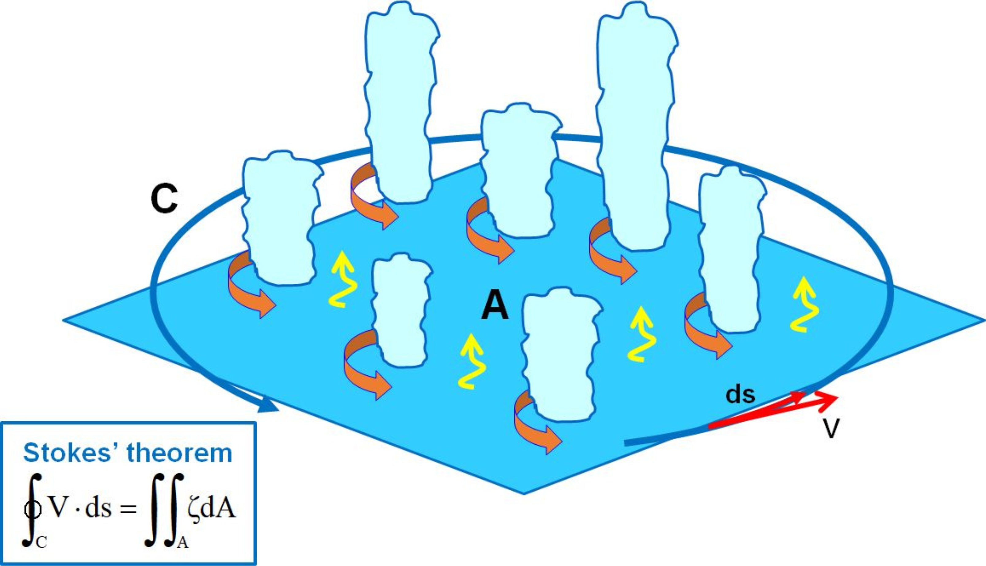
The dynamics of the rotating-convection paradigm are encapsulated, in part, by the azimuthal-mean tangential momentum equation, or equivalently by the vertical vorticity equation in conjunction with Stokes' theorem. Stokes' theorem equates the circulation about any fixed closed loop \(C\) to the area integral of the vorticity within that loop. Take \(A\) to be the area enclosed by loop \(C\) and the area to be in a horizontal plane, Stokes' theorem may be written in the form \begin{equation} \oint_C \mathbf{V} \cdot d\mathbf{s} = \int \int_A \zeta dA, \label{Eq1} \end{equation} where \(\mathbf{V}\) is the velocity vector, \(d\mathbf{s}\) is a vector increment along the curve \(C\), \(dA\) is an area element of \(A\), and \(\zeta\) is the vertical component of relative vorticity. There is a theorem by Haynes and Mcintyre (1987) showing that for the circulation about the circuit C to increase, implying that the mean tangential wind about this circuit increases, vertical vorticity must be brought horizontally into the region across the boundary of \(C\). A more general statement is that the change of horizontal circulation occurs via a line integral of a horizontal vorticity flux vector. The flux vector is the sum of an advective and non-advective component (see, e.g., Sections 2.15 and 11.1 of Smith and Montgomery, 2023). For simplicity, we focus here primarily on the advective vorticity flux component. These statements are the three-dimensional analogue of the idea that for spin up, the \(M\)-surfaces have to move inwards. It turns out that the local enhancement of vertical vorticity by vortex-line stretching in convective updraughts totally inside \(C\) does not increase the circulation about \(C\) because the amplification of vorticity is exactly compensated by the reduced area of the enhanced vorticity.
|
In a nutshell, the classical intensification theory may be invoked to understand the evolution of the azimuthally-averaged fields in a three-dimensional flow providing that the eddy-terms arising from departures from axial symmetry are taken into account in the formulation, or if these eddy terms are small enough to be neglected compared with the mean terms. Even if the eddy terms are not everywhere negligible, the classical theories provide useful qualitative insights into the physics of vortex evolution, even if the vortex is tilted in the vertical (Smith et al., 2017). Further details are provided in Chapter 11 of Smith and Montgomery (2023).
If there were no deep convection present, the convergence in the boundary layer would lead to divergence above the boundary layer and the circulation would weaken by the mechanism described in Section 3.6.2. Clearly,
The foregoing considerations offer insights into why tropical cyclogenesis is a relatively rare occurrence since genesis requires conditions favourable for deep convection to persist. Under normal circumstances, the cold pools produced by the evaporation of precipitation before it reaches the ground stabilize the region near the convection to future convection, although new convection might be triggered near the periphery of the cold pools (see e.g., Mapes 1993, Montgomery et al. 2006). The strength of downdraughts is increased by the presence of dry air in the low to mid troposphere where downdraughts originate. Given the chaotic nonlinear dynamics and thermodynamics of moist convection, there is clearly a stochastic element to this process.
For typical conditions over the warm tropical oceans, the cold pools, themselves, are removed by enthalpy fluxes from the sea, the time-scale for which depends on the local near-surface wind speed and the degree of disequilibrium between the specific humidity of near-surface air and the saturation specific humidity at the sea-surface temperature. Over the tropical oceans, this time-scale is typically on the order of half a day, but it reduces to one or two hours when near-surface winds become large as in tropical cyclones. In this way, the enthalpy fluxes, indicated in Figure 8, play a key role in restoring convective instability to guarantee the persistence of deep convection.
An important necessary condition for the formation of a tropical cyclone is the existence of a nearly closed circulation region (or “pouch”) in the disturbance-relative frame. For reasons summarized in Smith and Montgomery (2023, Section 1.5.5), a quasi-closed deep pouch spanning the lower troposphere supports the organization of the convection and vorticity around the centre of the pouch, the so-called “sweet spot” of the parent tropical disturbance. The pouch acts as a region protected from the intrusion of dry environmental air near the developing vortex core region, allowing deep and moderately deep convection to moisten its environment at levels where downdraught air originates in subsequent convection.
In summary,
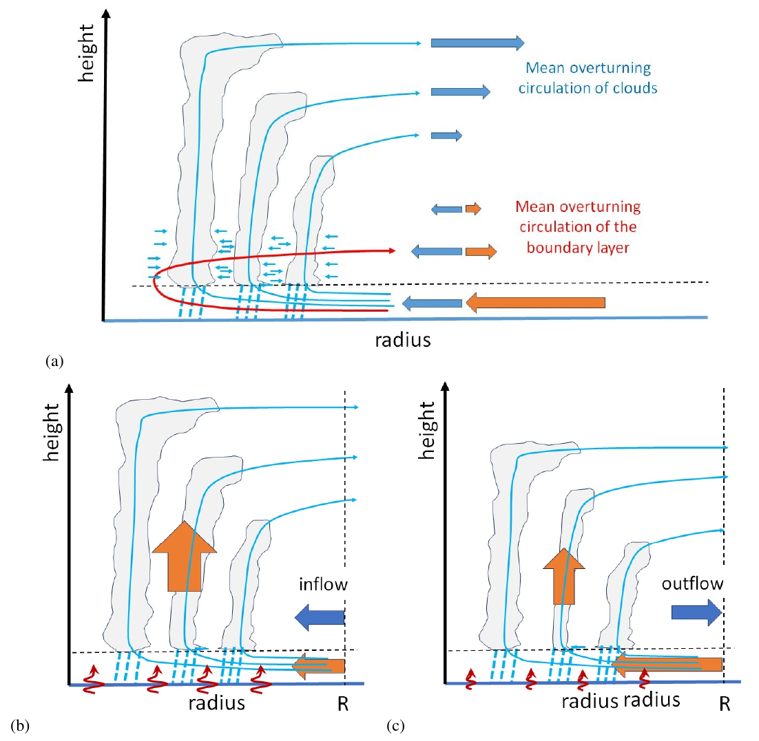
Smith et al. (2021) showed that the rotating-convection paradigm provides a useful framework for understanding much of the vortex behaviour during the entire life cycle. A central idea in this framework is the appreciation that the strength of deep overturning circulation induced by deep convection and the strength of the boundary layer inflow that supplies the convection with moist air are controlled by separate processes. Specifically,
During the genesis and rapid intensification stages of vortex evolution, the mass flux supplied by the frictional boundary layer to the inner core region of the vortex is outweighed by the mass flux carried upwards by the collective effects of deep convection (Figure 9b). As a result, the convectively-induced inflow in the lower part of the troposphere above the frictional boundary layer is strong enough to reverse the shallow layer of outflow that would otherwise be induced by the boundary layer (see e.g., Section 3.6). During these stages, the boundary layer is rapidly moistened by surface evaporation, the moistening being sufficient to maintain deep convective instability. In turn, moist convection in the core leads to a moistening of the vortex core region aloft, thereby reducing the strength of convective downdraughts in the core that would otherwise act to stabilize the boundary layer to further convection.
|
As a vortex matures, however, the inner core boundary layer comes closer to saturation, reducing the continued flux of surface moisture supply to maintain convective instability, whereas the upper levels of the vortex warm, a natural consequence of balance dynamics (e.g., Smith and Montgomery, 2024, Section 5.3). The upper-level warming has a stabilizing effect on inner-core deep convection and gradually gains the upper hand. As a result, the collective effects of deep convection become progressively less able to ventilate mass at the rate that mass is supplied by the boundary layer. This inability is enhanced by the increase in the boundary-layer mass flux as the vortex intensifies and broadens. The broadening is reflected, in part, by the progressive increase in the radius of maximum tangential wind speed as well as the increase in the radius of gales (see Smith et al., 2021, Figure 1). The broadening is, itself, a consequence of continued lower-tropospheric inflow above the boundary layer. Eventually, a situation is reached where convection is no longer able to ventilate all the mass converging in the boundary layer and the fraction that cannot be ventilated flows outwards in a shallow layer above the boundary layer (Figure 9c). When this happens, the tangential wind spins down locally, as in the friction only calculation discussed in Section 3.6, and the boundary layer flow weakens in response.
In the Smith et al. (2021) life-cycle simulation, the processes described above account also for a temporary decay and subsequent re-intensification of the vortex between about 9\(\frac12\) and 12 days. The decay is accompanied by a weakening of the mass flux carried by the inner eyewall convection and the resulting low-level outflow triggers a band of deep convection at larger radii. Subsequently, a new eyewall cloud forms at a larger radius than the original eyewall, but inside the band of deep convection. The re-intensification is accompanied by this new eyewall formation and the convection beyond it progressively decays.
The foregoing processes are broadly analogous to reducing the bubbling rate in the Turner-Lilly bubbling experiment, suitably modified for tropical cyclones as described in Section 3.3. One could imagine first reducing the bubbling rate from a ring of bubbling tubes and then increasing the rate while increasing the radius of the bubbling tubes. The additional effect in the foregoing numerical simulation is the stable stratification of the model atmosphere, which confines the unventilated radial outflow from the boundary layer to a shallow layer just above the boundary layer.
An important detail relating to vortex spin up in the rotating-convection paradigm is the so-called
If \(v\) does exceed \(v_g\) at some radius,
Whether or not \(v\) does actually exceed \(v_g\) at some inner radii can be ascertained only by doing a nonlinear boundary layer calculation or a full vortex simulation, although the foregoing considerations show this to be a plausible possibility. Indeed, many tropical cyclone simulations show that the maximum tangential wind is located within the strong inflow layer as do many recent observational analyses of real storms. In particular, both simulations and observations of intensifying and mature tropical cyclones show regions of supergradient flow as the air decelerates radially in the boundary layer and turns upwards into the eyewall (see Smith and Montgomery, 2023, Chapter 6).
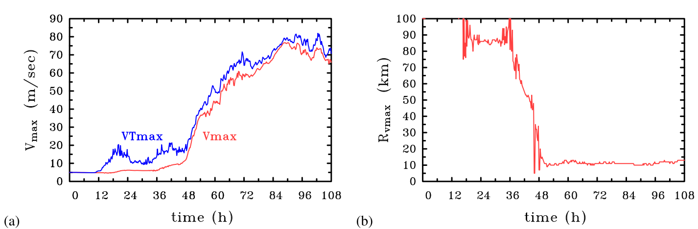
Figure 10 shows the evolution of the maximum azimuthally-averaged tangential wind speed, \(V_{max}\), the radius at which it occurs, \(R_{vmax}\), and the maximum total wind speed, (VT_{max}\), in a typical calculation starting from an initially cloud-free, balanced axisymmetric vortex on an \(f\)-plane. The details of this calculation may be found in Kilroy et al. (2017) and are summarized in Smith and Montgomery, 2023, Chapter 10.
|
The vortex evolution begins with a period of about 10 hours during which both \(VT_{max}\) and \(V_{max}\) decrease slightly because of friction. The imposition of surface friction at the initial time of the simulation reduces the tangential wind speed near the surface, elevating the height of the maximum. As explained in Smith and Montgomery, 2023, Chapter 6, this reduction leads to an inward agradient force in the layer affected by friction. The agradient force drives inflow in the shallow layer affected by friction and outflow just above the inflow layer. At this early stage, there is no deep convection to ventilate any of the inflowing air.
During the early spin down phase, the boundary layer moistens because of evaporation from the underlying sea surface. This moistening and the lifting of air within the boundary layer due to the frictionally-induced convergence reduce the convective inhibition (CIN) and increase the convective available potential energy (CAPE). These changes lead to convective instability and eventually to the initiation of isolated deep convective clouds. The rapid increase in \(VT_{max}\) a little after 12 hours is a result of the local overturning circulations accompanying these clouds. These local circulations break the axial flow symmetry of the initial vortex and account for the subsequent fluctuations of \(VT_{max}\). Before convection begins, the vortex remains close to axisymmetric, but thereafter the flow becomes markedly asymmetric. It is not until about 36 hours that \(V_{max}\) begins a marked increase also.
There is a turning point in the evolution at about 45 hours when \(V_{max}\) begins to increase more rapidly. At this time, \(V_{max}\) is only 9.1 m s−1 and \(VT_{max}\) = 17.4 m s−1. At 48 hours, there is a sharp rate of increase in both \(V_{max}\) and \(VT_{max}\). This time marks the onset of a period of
Stokes’ theorem discussed in Section 3.8.1 shows that the circulation about a fixed circuit in a flow is equal to the area mean of the vertical component of relative vorticity, \(\zeta\), enclosed by the circuit. It follows that the change in mean tangential wind speed about any circular contour in a vortical flow is equal to the change in mean vorticity enclosed by that circuit. For this reason it is of interest examine the evolution of vorticity as the vortex begins to intensify.
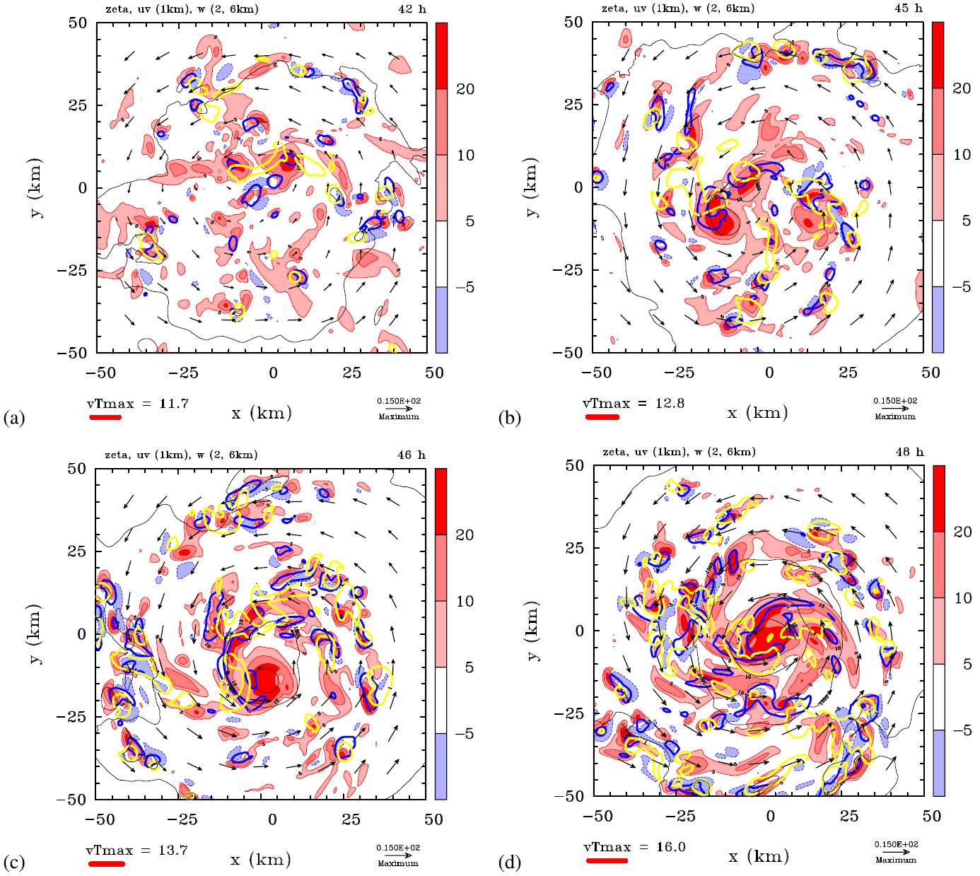
Figure 11 shows horizontal cross sections of \(\zeta\) in the central part of the fledgling vortex at selected times straddling the time 48 hours when intensification begins in earnest. Superimposed on each panel are the wind vectors at a height of 1 km, the isobars of surface pressure, and two 1 m s−1 contours of vertical velocity at different heights. The contours of vertical velocity, shown for heights of 2 km and 6 km, are chosen to indicate the location of strong updraughts at these levels. Where these contours overlap or lie in close proximity gives an indication of the location of vertically coherent or possibly sloping deep convective updraughts. Panel (a) shows the fields at 42 hours, six hours before intensification begins in earnest, while subsequent panels show the fields at 45 hours (panel (b)), 46 hours (panel (c)), and finally at 48 hours (panel (d)) when RI begins (see Figure 10).
At 42 hours (panel a), there are several irregular-shaped patches of locally-enhanced cyclonic vertical vorticity, the ones largest in area lie in a west-southwest to eastnortheast-oriented strip to the north of the vortex centre and in a sector to the south west of the vortex centre. (We refer to the coordinate directions using geographical descriptions, the horizontal coordinate in the figure pointing east and the vertical coordinate pointing north.) These patches result from the stretching of ambient vortex vorticity by previous as well as current deep convective cells. The circulation centre at 42 hours, indicated by the velocity vectors, lies near the centre of the computational grid, while the surface pressure field is quite diffuse at this time. In fact, the location of minimum pressure is not apparent at the 2 mb contour spacing shown. The value of \(V_{max}\) is 9.0 m s−1, while that of \(R_{vmax}\) has reduced from 100 km at initial time to 55 km (Figure 10).
There are a few patches of negative (anticyclonic) vertical vorticity also. These are associated with the tilting of horizontal vorticity into the vertical by convective updraughts and downdraughts, which tends to produce dipole structures. A few such dipoles are evident beneath strong updraught roots at 2 km height, for example near (−20 km, 35 km), (43 km, −2 km), and (34 km, −12 km).
At 45 hours (panel (b)), the centre of circulation remains within about 10 km of the centre of coordinates and the surface pressure field remains diffuse. The value of \(V_{max}\) has risen by only 0.2 m s−1, but generally the winds have strengthened near the circulation centre and there has been a marked aggregation of cyclonic relative vorticity. Individual patches of cyclonic vorticity have increased in size and have begun to consolidate around the vortex centre. In particular, the area of patches with a magnitude exceeding > 1 × 10⁻³ s−1 has increased. There are many patches of negative vertical vorticity also, but again, these occur mostly on the periphery of the coherent region of cyclonic vorticity that surrounds the centre of circulation. The regions with updraught speeds exceeding 1 m s−1 at a height of 6 km (the areas enclosed by yellow contours in the figure) have increased markedly in area over the previous three hours, indicating that deep convection has become more widespread.
By 46 hours (panel (c)), the cyclonic vorticity surrounding the centre of circulation has consolidated further and there is a significant updraught region at 6 km height near the region with the largest area of elevated cyclonic vorticity. Although \(V_{max}\) at this time has increased by only 0.9 m s−1 in one hour, a small closed contour of surface pressure has formed near the centre of circulation indicating that the pressure has started to fall within the central core of high cyclonic vorticity. At this time, the circulation centre has moved about 12 km south of the centre of coordinates.
Two hours later, at 48 hours (panel (d)), the monopole of high cyclonic vorticity near the centre of circulation has grown in size and \(V_{max}\) has increased to 14.0 m s−1. Similar plots at later times portray an acceleration of the intensification process with the appearance of more and more concentric surface isobars.
Despite the relatively simple configuration of the foregoing thought experiment, the flow evolution becomes rather complex in detail. The complexity is largely because of the formation of deep convective clouds, which introduces a stochastic element to the evolution. Compounding the complexity of the processes involved, the moist thermodynamics of the transition to a self-sustaining, coherent, convective vortex entails subtle, but important changes in the thermodynamic structure of the flow near the emergent centre of circulation (See Smith and Montgomery, 2023, Sections 10.4, 10.5 and 10.11).
|
Click here for a movie of the fields in Figure 11 including a depiction of the three-dimensional structure of deep convection.
A cartoon summarizing the azimuthally-averaged aspects of the rotating-convection paradigm for tropical cyclogenesis and intensification in a favourable environment is shown in Figure 12. The depiction highlights the role of localized, rotating deep convection that grows in the cyclonic, rotation-rich environment of the incipient storm, structures that are intrinsically three dimensional. The convective updraughts greatly amplify the vertical vorticity locally by vortex-tube stretching, and the patches of enhanced cyclonic vorticity subsequently aggregate to form a central monolith of cyclonic vorticity, the aggregation being facilitated mainly by the axisymmetric-mean overturning circulation associated with the convection, itself. Convective instability is maintained principally by latent heat fluxes at the air-sea interface, which are enhanced as the near-surface wind speed increases. The stochastic nature of deep convection arising from the instability means that local asymmetric features of the developing vortex have limited predictability.
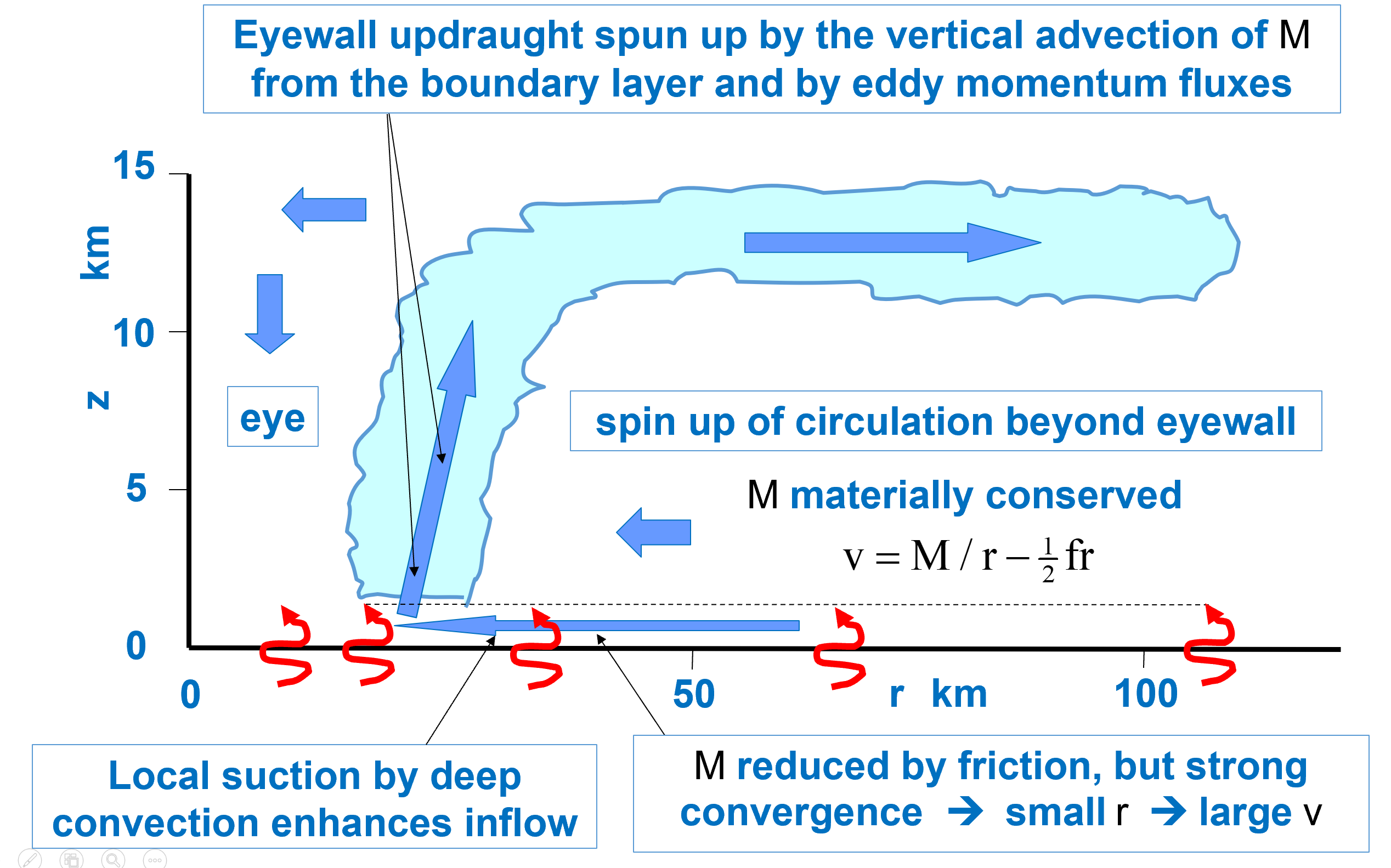
|
This azimuthally-averaged perspective shares many elements of the classical paradigm for spin up summarized in Section 3.7.5. There is inflow in the lower troposphere, above the boundary layer. This inflow is attributed to the collective effects of buoyancy generation by latent heat release in the inner-core deep convection. There is ascent in the heated region and outflow in the upper troposphere. Further, because absolute angular momentum is approximately materially conserved in the outflow layer, the tangential velocity becomes anticyclonic beyond a certain radius. This anticyclone is not shown in Figure 12 due to the limited horizontal domain chosen for highlighting the inner core structure.
A feature in Figure 12 that is not part of the classical paradigm is the occurrence of the maximum tangential wind speed in the layer of strong, low-level inflow. Although the strong inflow is associated primarily with the reduction of the tangential wind by the frictional stress at the ocean surface, the occurrence of the maximum tangential wind within the frictional boundary layer is a result of the nonlinear boundary layer spin up enhancement mechanism that operates in the inner core region. In addition to this boundary layer mechanism, there is a suction effect of the convection in the boundary layer which further enhances the inflow near and beneath the eyewall cloud complex. Because of the nonlinearity of the dynamical equations in this region, these two effects cannot be isolated in general.
Since the flow is not axisymmetric, especially during the genesis and early intensification phase of evolution, the azimuthally-averaged description is incomplete unless the spatial-temporal structure of the eddy processes is known. This structure can be diagnosed from the complete solution (see Persing et al. 2013 and Smith and Montgomery, 2023, Chapter 11).
To reiterate,
Links to two movies illustrating the evolution of the azimuthally-averaged flow in two published simulations of tropical cyclones are found below.
Click here for a movie of the fields from the genesis simulation in Kilroy et al. (2017).
Click here for a movie of the fields from the life-time simulation in Smith et al. (2021).
All the movies in Section 3.8 with a full description may be found on the companion website to our textbook: Smith and Montgomery, 2023, "Tropical cyclones: Observations and Basic Processes", see Chapter 10.
The foregoing presentation has focussed on the prototype problem for tropical cyclone evolution in a quiescent environment. One omission so far is the topic of secondary eyewall formation and behaviour. A further omission is an extension to environments that are not quiescent, such as ones with a uniform flow or uniform shear flow. Work to address these omissions is continuing.
I gratefully acknowledge perceptive comments and suggestions from my colleague, Mike Montgomery, in constructing this page. The foregoing discussion is based in part on a recent paper that we coauthored (Smith and Montgomery, 2024).
Bui, H. H., R. K. Smith, M. T. Montgomery, and J. Peng, 2009: Balanced and unbalanced aspects of tropical-cyclone intensification. Quart. J. Roy Met. Soc. 135, 1715-1731.
Črnivec, N., R. K. Smith, and G. Kilroy, 2016: Dependence of tropical cyclone intensification rate on sea surface temperature. Quart. J. Roy. Meteor. Soc., 142, 1618-1627.
Eliassen, A., 1951: Slow thermally or frictionally controlled meridional circulation in a circular vortex. Astroph. Norv., 5, 19-60.
Eliassen, A., 1962: On the vertical circulations in frontal zones. Geofys. Publ., 24, 147-160.
Eliassen, A., 1971: On the Ekman layer in a circular vortex. J. Meteor. Soc. Japan, 49, 784-789.
Eliassen, A. and M. Lystad, 1977: The Ekman layer of a circular vortex: A numerical and theoretical study. Geophys. Norv., 31, 1-16.
Haynes, P., and M. E. McIntyre, 1987: On the evolution of vorticity and potential vorticity in the presence of diabatic heating and frictional or other forces. J. Atmos. Sci., 44, 828–841.
Kilroy, G., R. K. Smith, and M. T. Montgomery, 2017: A unified view of tropical cyclogenesis and intensification. Quart. Journ. Roy. Meteor. Soc., 143, 450–462.
Mapes, B.E., 1993. Gregarious tropical convection. J. Atmos. Sci. 50, 2026–2037.
Montgomery, M. T. and R. K. Smith, 2011: Tropical cyclone formation: Theory and idealized modelling. In Proceedings of Seventh WMO International Workshop on Tropical Cyclones (IWTC-VII), La ReUnion, Nov. 2010. (WWRP 2011-1) World Meteorological Organization: Geneva, Switzerland, 87, in press.
Montgomery, M. T. and R. K. Smith, 2014: Paradigms for tropical cyclone intensifcation. Aust. Met. Ocean. Soc. Journl., 64, 37-66.
Montgomery, M. T., and J. Persing, 2020: Does balance dynamics well capture the secondary circulation and spinup of a simulated hurricane? J. Atmos. Sci., 78, 75–95.
Montgomery, M. T., M. E. Nichols, T. A. Cram, and A. B. Saunders, 2006: A vortical hot tower route to tropical cyclogenesis. J. Atmos. Sci., 63, 355–386.
Morton, B. R., 1966: Geophysical vortices, In Prog. In Aeronautical Sci., Ed. Küchemann, Vol. 7. Pergamon, 145-194pp
Ooyama, K. V., 1969: Numerical simulation of the life cycle of tropical cyclones. J. Atmos. Sci., 26, 3-40.
Ooyama, K.V., 1982. Conceptual evolution of the theory and modeling of the tropical cyclone. J. Meteorol. Soc. Japan. 60, 369–380.
Ooyama, K. V., 1997: Footnotes to "Conceptual evolution". Extended abstracts, 22nd Conference on Hurricanes and Tropical Meteorology, American Meteorological Society, Boston, 60, 13-18.
Persing, J., M. T. Montgomery, J. McWilliams, and R. K. Smith, 2013: Asymmetric and axisymmetric dynamics of tropical cyclones. Atmos. Chem. Phys., 13, 12 299-12 341.
Schubert, W. H., and B. T. Alworth, 1982: Evolution of potential vorticity in tropical cyclones. Quart. Journ. Roy. Meteor. Soc., 39, 1687–1697.
Schubert, W. H., and J. J. Hack, 1983: Transformed Eliassen balanced vortex model. J. Atmos. Sci., 40, 1571–1583.
Shapiro, L. J. and H. Willoughby, 1982: The response of balanced hurricanes to local sources of heat and momentum. J. Atmos. Sci., 39, 378-394.
Smith, R. K., and L. M. Leslie, 1976: Thermally driven vortices: a numerical study with application to dust devils. Quart. Journ. Roy. Meteor. Soc., 102, 791–804.
Smith, R. K., and M. T. Montgomery, 2016: Understanding hurricanes. Weather, 71, 219-223.
Smith, R. K., and M. T. Montgomery, 2023: Tropical cyclones: Observations and basic processes. Elsevier, London, 411pp.
Smith, R. K., and M. T. Montgomery, 2024: Towards understanding the tropical cyclone life cycle. Tropical Cyclone Research and Review, 13, In press.
Smith, R. K., M. T. Montgomery, and S. V. Nguyen, 2009: Tropical cyclone spin up revisited. Quart. Journ. Roy. Meteor. Soc., 135, 1321-1335.
Smith, R. K., G. Kilroy, and M. T. Montgomery, 2015: Why do model tropical cyclones intensify more rapidly at low latitudes? J. Atmos. Sci., 72, 1783-1804.
Smith, R. K., J. A. Zhang and M. T. Montgomery, 2017: The dynamics of intensification in an HWRF simulation of Hurricane Earl (2010). Quart. J. Roy. Meteor. Soc., 143, 293-308.
Smith, R. K., M. T. Montgomery, and H. Bui, 2018: Axisymmetric balance dynamics of tropical cyclone intensification and its breakdown revisited. J. Atmos. Sci., 75, 3169–3189.
Smith, R. K., M. T. Montgomery, and S. Wang, 2024: Can one reconcile the classical theories and the WISHE-theories of tropical cyclone intensification? Tropical Cyclone Research and Review, 13, In press.
Turner, J. S., and D. K. Lilly, 1963: The carbonated-water tornado vortex. Quart. Journ. Roy. Meteor. Soc., 20, 468–471.
Wang, S. and R. K. Smith, 2019: Consequences of regularizing the Sawyer-Eliassen equation in balance models for tropical cyclone behaviour. Quart. Journ. Roy. Meteor. Soc., 145, 3766–3779.
Wang, S., R. K. Smith and M. T. Montgomery, 2020: Upper-tropospheric inflow layers in tropical cyclones. Quart. J. Roy. Meteor. Soc., 146, 3466-3487.
Wang, S., M. T. Montgomery, and R. K. Smith, 2021: Solutions of the Eliassen balance equation for inertially and/or symmetrically stable and unstable vortices. Quart. J. Roy. Meteor. Soc., 146, 2760-2771.
Willoughby, H. E., 1979: Forced secondary circulations in hurricanes. J. Geophys. Res., 84, 3173–3183.
Latest version: Munich 3 January 2025