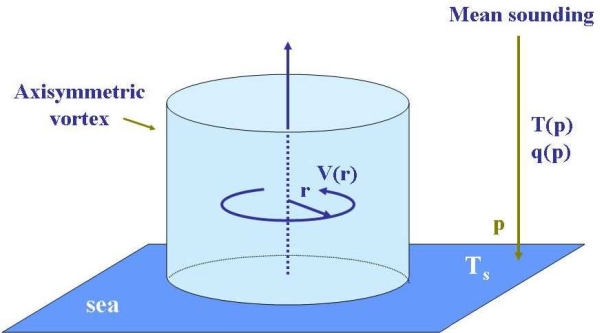
Here we develop a three-layer, axisymmetric, numerical model to explore basic aspects of vortex amplification in the prototype problem for tropical cyclone intensification, illustrated in Fig. 6.1. This problem considers the evolution of an initially cloud-free, symmetric vortex in a quiescent environment on an f-plane with an environmental sounding typical of the tropical-cyclone season. The sea surface temperature, Ts, is prescribed. The vortex is assumed to be in thermal wind balance. The balanced temperature field is obtained by the method described in Chapter 3. The model is a minimal one in the sense that it contains only the essential processes that are required to develop a reasonably realistic tropical cyclone. Even then the problem is too complicated to solve analytically and we must resort to numerical methods. Here we use a finite-difference approach. We assume that the reader is broadly familiar with the principal features of such an approach. The discretization in the vertical has just three layers, the minimum number required to represent the near-surface inflow layer in which surface frictional effects are important, a lower tropospheric layer in which convectively-induced inflow may take place, and an upper-tropospheric outflow layer.
A particular challenge in the development of the minimal model is the representation of deep convection, the so-called cumulus parameterization problem. This problem is circumvented in VVV, where the same prototype problem is studied using a more sophisticated multi-layer model in which deep convection is explicitly resolved. Even so, the minimal model and the representation of deep convection therein is instructive.
The numerical model uses the hydrostatic primitive equations in cylindrical sigma-coordinates (r, λ, σ) on an f-plane, where

p^* = p_s - p_{top}, p_s and p_{top} are the surface and top pressures, and p_{top} is a constant, taken here to be 100 mb. Then the upper and lower boundary conditions require that \dot σ = 0 at σ = 0 and σ = 1, where \dot σ = Dσ /Dt is the vertical σ-velocity, t is the time, and D/Dt is the material derivative. The radial and tangential momentum equations and the hydrostatic equation are:
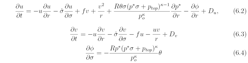
where u and v are velocity components in the radial r- and azimuthal λ-directions, φ is the geopotential, and Du and Dv represent the frictional drag in the r- and λ-directions, respectively, and other quantities have been defined previously. The specification of Du and Dv is given in an Appendix. The surface pressure tendency equation, derived from the continuity equation and boundary conditions is

and \dot σ is given by

The thermodynamic and moisture equations are

and

where h_d is the dry static energy (see section XX), q is specific humidity, Q_{h_d} and Q_q represent the diabatic heat and moisture sources, respectively, including those associated with deep cumulus convection. The temperature T is related to h_d by
\begin{equation}\label{eq6.9} T =\frac{h_d - gz}{c_p}. \end{equation}
Newtonian cooling is added in the thermodynamic equation to represent the effect of radiative cooling. The idea is to relax temperature to the ambient temperature on a prescribed time scale. \textbf{discuss why} The turbulent flux of momentum to the sea surface and the fluxes of sensible heat and water vapour from the surface are represented by an empirical bulk formulae. The surface drag is represented by (\textbf{earlier equation?}):
\begin{equation} \taus = \rho C_D |\mathbf{u_b}|\mathbf{u_b}, \end{equation}where C_D is a drag coefficient and \mathbf{us} = (us,vs). This term represents the rate of which momentum is lost to the surface and characterizes the frictional drag imposed by the surface on the air above. A similar law is taken for the enthalpy and moisture fluxes:

where χ_s and χ_{surf} are the values of χ in the air just above the sea surface, normally taken to be at a height of 10 m, and at the sea surface, respectively. In the case of temperature χ_s is the sea surface temperature and in the case of moisture it is the saturation specific humidity at this temperature. Based on the latest available data we use the formula C_D = C_{D0} + C_{D1}|\bf{u_b}|, where C_{D0} = 0.7 \times 10^{-3} and C_{D1} = 6.5 \times 10^{-5} for wind speeds less than 20 m s-1 and C_{D} = 2.0 \times 10^{-3}. We take C_{χ} to be a constant with the value 1.1 \times 10^{-3}.
The calculations are carried out in a cylindrical domain ({0 \leq r \leq R,\,\,0 \leq σ \leq 1} ) with the following boundary conditions:
\begin{equation}\label{eq5.10n} u = 0,\quad v = 0,\quad \frac{{\partial A}} {{\partial r}} = 0,\quad at \quad r=0, \end{equation}and
\begin{equation}\label{eq5.11n} u = 0,\quad v = 0,\quad \frac{{\partial A}} {{\partial r}} = 0,\quad at \quad r=R \end{equation}where A can be any of the quantities u, v, hd, q. The former expresses a symmetry condition at the axix of rotation and the latter takes the outer boundary to be a rigid wall. The initial axisymmetric vortex is baroclinic and the azimuthal velocity distribution is detailed given by
\begin{equation}\label{eq5.11n} v(r,z) = specify \end{equation}It has a maximum wind speed of 15 m s-1 at a radius of 120 km.
The corresponding thermal field, surface pressure, and geopotential are obtained by the method outlined in Chapter 3.
The far-field temperature and humidity structure are based on the mean West Indies sounding for the `hurricane season' (Jordan, 1957), but the near-surface mixing ratio has been reduced slightly so that the sounding is initially stable to deep convection. The initial surface pressure is 1015 mb. In the presence of the initial vortex, the minimum surface pressure (at the vortex centre) is 1008 mb. Horizontal variations of mixing ratio in the presence of the initial vortex are neglected. Details of the initial sounding are given in the appendix (add link).

The model is divided vertically into three unequally deep layers with boundaries at σ = 1, σ_4, σ_2 and 0 (see Fig. \ref{Fig6.2}). All the dependent variables, such as horizontal velocity, potential temperature, specific humidity and geopotential, are defined in the middle of each layer (σ = σ_b, σ_1, and σ_3), and the vertical velocity is staggered, i.e. it is defined at the boundaries between layers. The variables are staggered in the radial direction also as indicated in Fig. 6.2. The equations are expressed in finite difference form in both the horizontal and vertical and integrated using the Adams-Bashforth third-order method. The initial pressure, temperature, mixing ratio and geopotential height in the middle of each layer and at the boundaries between layers are listed in the appendix.
An important consideration in tropical cyclone modelling is the suppression of small-scale noise and numerical instability in the calculations. This problem becomes of extreme importance when the formulation provides for the explicit release of latent heat. The methods used in this paper are detailed in an appendix (add link).
Explicit condensation is treated in the simplest possible way. If at any time the air becomes saturated at a grid point, grid-scale condensation and precipitation processes are allowed. The excess water vapour is condensed to liquid water and is assumed to precipitate out, while the latent heat released is added to the air. The resulting increase in air temperature raises the saturation vapour pressure so that the parcel is no longer saturated and a small fraction of the condensed water must be re-evaporated. This evaporation again lowers the air temperature and the vapour pressure and an iteration is required to find the precise saturation temperature. In practice this procedure requires only a few iterations. This procedure is applied before the sub-grid-scale convection scheme, whereupon the convection scheme to be described is always applied to a conditionally-unstable atmosphere with relative humidity less than 100% (n.b. if the relative humidity equals 100%, the condition for convective instability discussed below is not satisfied).
At the time of writing, all global numerical models used for forecasting tropical cyclones have a horizontal resolution that is too coarse to resolve cumulus clouds. That means that the effects of such clouds, which are subgrid scale, must be parameterized in terms of those quantities that are carried in the model. We refer to this as the cumulus parameterization problem. A number of ways to parameterize clouds has been suggested and a review of these is contained in references given at the end of this chapter. We shall consider one type of scheme here, the so-called mass-flux scheme, in which clouds are represented as entraining columns of ascending air covering a part of a grid box with adjacent columns of descending air representing downdrafts. Deep clouds take air form the boundary layer and expel (or detrain\footnote{The word ``detrainment" has become commonly used to describe the expulsion of air from convective clouds, whereas ``entrainment" is used to describe the process whereby ambient air is incorporated into clouds by mixing. Strictly, these terms are not opposites, since entrainment is not a reversible process.}) it into the upper troposphere, the so-called \textit{detrainment layer}.

The exchange of mass between a deep convective cloud and its environment within a grid column, and the exchange between adjacent grid columns is shown schematically in Fig. 6.3, for the case of two-dimensional flow in the {x-σ} plane. For the purpose of illustration only, all the mass exchange between adjacent grid cells is taken to occur through the boundary on the right of the grid column (x = Δ x) and we consider the case in which the dependent variables are horizontally staggered with u_n stored on the boundary and other variables in the middle of a grid cell. In the present model, where the variables are not horizontally staggered, the configuration shown would apply to two adjacent grid columns. The subgrid-scale vertical transports are formulated by considering the cloudy and clear-air regions of the grid column separately. The subgrid-scale fluctuations in the dependent variables are associated with different (uniform) values of these quantities in these regions. \textit{Deep convection is assumed to occur in a grid column if the moist static energy in the boundary layer} h_b \textit{exceeds the saturation moist static energies in the upper and lower troposphere}, h_1^* and h_3^* (Henceforth, a star denotes the saturation value of a thermodynamic variable). The vertical mass transfer between parts of grid cells is characterized by a mass flux per unit area with magnitude M = |p^*<\dot σ>/g| and units \mathrm{kg s-1 m-2}. The positive sign of M is different in different parts of a grid box as indicated in Fig. 6.3. The resolved-scale averaged mass fluxes \overline M_{n} at levels-2 and ?4 are assumed to be positive for ascending motion.
The mass-flux method assumes a steady-state bulk cloud model, indicated by the cloud on the left of the diagram in Fig. 6.3. In the cloud model, M_{c4} is the cloud-base mass flux from the boundary layer to the middle layer, M_e is mass flux entrained into the cloud from the middle layer, and M_{c2} is the mass flux transferred from the middle layer to the upper layer inside the cloud (here a subscript {`}c{'} denotes a cloud property). Continuity of mass requires that
\begin{equation} M_{c2}=M_{c4}+M_e . \label{eq3-6} \end{equation}We assume that air which detrains from the cloud into layer-1 has zero buoyancy so that, although it is saturated, its temperature is the same as that of the environment in layer-1. Then
\begin{equation} M_{c2}h_{c1}=M_{c4}h_b+M_eh_3 . \label{eq3-7} \end{equation}where h_{c1}= h_1^* is the saturation moist static energy of cloudy air in layer-1. As shown below, Eq. (\ref{eq3-7}) determines the mass flux entrained into the cloud. Combining (\ref{eq3-6}) and (\ref{eq3-7}), and writing
\begin{equation} M_{c2}=\eta M_{c4} , \label{eq3-9} \end{equation}we obtain
\begin{equation} \eta = 1 + {{h_b-h_1^*} \over {h_1^*-h_3}} \label{eq3-10} \end{equation}and it follows using Eq. (\ref{eq3-6}) that
\begin{equation} M_e=(\eta -1)M_{c4} \label{eq3-11} \end{equation}Note that the condition for deep convection (h_b > h_1^*) ensures that the entrainment mass flux given by Eq. (\ref{eq3-11}) is positive, provided that h_1^* > h_3; i.e. the atmosphere is stable with respect to middle-level convection. This condition is always satisfied in the present calculations.
\subsection{Subgrid-scale mass fluxes in the clear air} It is assumed that precipitation falls into the cloud environment in layer-3 and that a precipitation-cooled downdraft brings air with the moist static energy of that layer into the boundary layer. Let M_{d4} be the downdraft mass flux from the middle layer to the boundary layer. Following Emanuel (1995a) we take the downdraft mass flux proportional to the updraft mass flux, i.e. \begin{equation} M_{d4}=χ M_{c4} , \label{eq3-8} \end{equation} where the quantity χ is linked to the precipitation efficiency \varepsilon through the expression χ~=~1 - \varepsilon. Emanuel (1995a) relates \varepsilon to the relative humidity of the middle layer in a way that downdrafts are stronger when the middle layer is relatively dry and weaker when it is relatively moist. For a similar reason we define \varepsilon~=~q_3/q_3^*, where q_3^* is the saturation specific humidity in layer-3. Note that 0\le χ \le 1. Since the grid-averaged vertical velocity at each level is the sum of the average cloud and cloud environment mass fluxes within the grid box, the mass fluxes at levels-2 and -4 in the cloud environment are M_{c2}-\overline M_2 and M_{c4}-\overline M_4, respectively. The latter may be subdivided into an amount M_{d4} that occurs in precipitation and an amount M_{e4} = M_{c4}-M_{d4}-\overline M_4 that occurs in clear air (see Fig.2). Then, in the cloud-free environment in unit time, M_{c2}h_{c1} units of h are detrained from the cloud to layer-1 and (M_{c2}-\overline M_2)h_2 units are transferred from this layer to layer-3 by the return circulation associated with the clouds. Altogether, (M_{e4}h_4 + M_{d4}h_3) units of h are transferred from the middle layer to the boundary layer, partly as subsidence in precipitation-free air (the first term in this expression) and partly in precipitation-cooled downdrafts (the second term). Note that \textit{(saturated) downdrafts in our model have a larger effect on the boundary layer moist static energy budget per unit mass transferred than subsidence in precipitation-free air, as the origin of downdraft air is higher and the moist static energy lower}. This is different from Emanuel's 1989- and 1995-formulations, where the moist entropy of downdraft air and subsiding clear air are the same. It is important to note that, while in many circumstances the precipitation-free, intra-cloud air will be subsiding (i.e. M_{e4} > 0), this does not have to be the case and we shall show that regions of ascent may and do occur (i.e. M_{e4} < 0). \subsection{Subgrid-scale heat and moisture sources} The six equations governing the convection scheme consist of prognostic equations for the dry static energy, s (= c_pT + φ), and q in each layer. Then the moist static energy, h = s + Lq. The formulation of the equations is essentially the same as that given by Arakawa (1969) and reproduced in the book by Haltiner (1971; see section 10.4), although both authors focus on the closure for middle-level convection, the conditions for which are never met in our model. The basis of the derivation is sketched briefly in Appendix C. The assumption that the fractional coverage of convective cloud, μ, in a grid column is small compared with unity enables the grid-averaged changes of these quantities to be approximated with the changes that occur in the cloud environment. Because the grid-scale and subgrid-scale vertical mass fluxes at any level are not independent (see subsection (c) above), the formulation of the source terms and vertical advection terms in Eqs. (7) and (8) need to be considered together wherever deep convection is called for in a grid column. Application of the volume-averaged conservation equation derived in Appendix C and the assumption that the cloud-environment mean of q and s is approximately equal to the mean over the entire grid cell leads to the following equations the rates-of-change of q and s in the top, middle, and boundary layer as a result of subgrid-scale fluxes: \begin{equation} \alpha _1p^*{{\partial q_1} \over {\partial t}}=M_{c2}\left( {q_{c1}-q_1} \right)-\left( {M_{c2}-\overline M_2} \right)\left( {q_2-q_1} \right), \label{eq3-12} \end{equation} \begin{equation} \alpha _3p^*{{\partial q_3} \over {\partial t}}=\left( {M_{c2}-\overline M_2} \right)\left( {q_2-q_3} \right)-M_{d4}\left( {q_{d4}-q_3} \right)-\left( {M_{c4}-M_{d4}-\overline M_4} \right)\left( {q_4-q_3} \right), \label{eq3-13} \end{equation} \begin{equation} \alpha _bp^*{{\partial q_b} \over {\partial t}}=M_{d4}\left( {q_{d4}-q_b} \right)+\left( {M_{c4}-M_{d4}-\overline M_4} \right)\left( {q_4-q_b} \right), \label{eq3-14} \end{equation} \begin{equation} \alpha _1p^*{{\partial s_1} \over {\partial t}}=-\left( {M_{c2}-\overline M_2} \right)\left( {s_2-s_1} \right), \label{eq3-15} \end{equation} \begin{equation} \alpha _3p^*{{\partial s_3} \over {\partial t}}=\left( {M_{c2}-\overline M_2} \right)\left( {s_2-s_3} \right)-M_{d4}\left( {s_{d4}-s_3} \right)-\left( {M_{c4}-M_{d4}-\overline M_4} \right)\left( {s_4-s_3} \right), \label{eq3-16} \end{equation} \begin{equation} \alpha _bp^*{{\partial s_b} \over {\partial t}}=M_{d4}(s_{d4}-s_b)+\left({M_{c4}-M_{d4}-\overline M_4} \right)(s_4-s_b), \label{eq3-17} \end{equation} where q_{c1} is the specific humidity of cloudy air in layer-1; s_{d4} and q_{d4} are the dry static energy and specific humidity of downdraft air as it crosses level-4; \alpha _n=Δ σ _n/g, where Δ σ_n, (n = 1, 3, b) are the thicknesses of layers-1, -3 and -b in terms of σ; and s_2, s_4, q_2, q_4 are obtained from values of s and q at adjacent levels by interpolation (the details are explained in Appendix B). We have included the grid-scale vertical fluxes in these equations to emphasize that they determine the \textit{net} vertical motion in the cloud environment, but they, together with the grid-scale horizontal transports, are calculated in Eqs. (\ref{eq2-7}) and (\ref{eq2-8}) and the subgrid-scale increments to q and s are calculated from Eqs. (\ref{eq3-12}) - (\ref{eq3-17}) with the grid-scale vertical mass transports excluded. The heating contributions from deep convection to Q_{\theta} in Eq. (\ref{eq2-7}) are obtained by calculating the increments in dry static energy, Δ s_n, during a time step, using Eqs. (\ref{eq3-15}) - (\ref{eq3-17}) with the terms involving the grid-scale mean quantities \overline M_2 and \overline M_4 \textit{excluded}. Then we set Q_{\theta n}=Δ s_n/(c_p\pi_n), where \pi _n is the Exner function at the appropriate σ-level (n = 1, 3, b). The moistening contributions Q_q in Eq. (\ref{eq2-8}) are obtained in a similar way using Eqs. (\ref{eq3-12}) - (\ref{eq3-14}). When downdrafts are excluded, Eqs. (\ref{eq3-12}) - (\ref{eq3-17}) are identical to those given by Arakawa (1969). It remains now to calculate the values of s_{d4}, q_{d4} and M_{c4}. The calculation of s_{d4} and q_{d4} is described in subsection (e) below. A closure assumption is required to determine the cloud-base mass flux, M_{c4}. The three methods explored here are described in subsections (f)-(h). \subsection{Downdraft thermodynamics} The calculation of s_{d4} and q_{d4} is indicated schematically in Fig. 3. It is assumed that rain falls into the air in layer-3 and partially evaporates until the air at this level becomes saturated and cooled to the wet-bulb temperature, T_{w3}. Then it is assumed that the cooled air descends into the boundary layer as rain continues to evaporate into it so as to just keep it saturated. The wet-bulb temperature at level-4, T_{w4}, is calculated by solving iteratively the equation \begin{equation} c_pT_{w4}+gz_4+Lq^*(T_{w4},p_4)=h_3, \label{eq3-18} \end{equation} and the specific humidity at level-4, q_{w4}, is simply equal to q^*(T_{w4},p_4). Since the moist static energy of an air parcel is approximately conserved when liquid water evaporates into it as well as during saturated descent, downdrafts reduce the moist static energy of the boundary layer. Further, because the moist static energy of downdraft air at level-4 is less than that of precipitation-free air at this level, downdraft air is more effective in decreasing the boundary layer moist static energy than subsidence in precipitation-free air. This representation of downdrafts leads to the coldest boundary-layer temperature that can be achieved by precipitation-cooled subsidence. In reality the evaporation of precipitation normally insufficient to keep downdrafts saturated, and this diminishes their cooling and moistening effect. \begin{figure} [!ht] \begin{center} \includegraphics[width=0.70\textwidth]{Figs/Fig5.0X.eps} \end{center} \caption{Schematic diagram showing how the downdraft temperature is determined. First, water is added to air parcels at level-3 until they are saturated. This lowers the temperature to the wet-bulb temperature T_{w3}, but increases the specific humidity to q^*_{w3}. It is assumed then that the parcels descend as precipitation continues to evaporate into them to keep them just saturated. The saturation moist static energy is approximately conserved during this descent.} \label{Fig5.02} \end{figure} \vspace{0.5cm} There are three different options in the model for representing subgrid-scale deep cumulus convection. The first is a modified version of the scheme proposed by Arakawa in 1969. The modified form of Arakawa{'}s scheme described here includes the effects of precipitation-cooled downdrafts. The second scheme is based on the boundary-layer quasi-equilibrium scheme used by Emanuel (1995a), but differs from the original Emanuel scheme in certain important details as described in section (g) below. The third scheme assumes that the (net) cloud-base mass flux is proportional to the resolved-scale vertical velocity at the top of the boundary layer, but it includes also the effects of precipitation-cooled downdrafts. In fact, the only difference between the three schemes as implemented here lies in the closure assumption that determines the cloud-base mass flux. \subsection{The modified 1969 Arakawa scheme} The closure for this scheme is obtained by assuming that deep convection tends to reduce the instability on the time, \tau_{dc}, and in doing so drives the moist static energy of the upper layer towards that of the boundary layer. Mathematically we write \begin{equation} p^*{\partial \over {\partial t}}\left( {h_b-h_1^*} \right)=-{{p^*(h_b-h_1^*)} \over {\tau _{dc}}} . \label{eq3-19} \end{equation} It can be shown that (see e.g. Haltiner, 1971, p189) \begin{eqnarray} p^*{\partial \over {\partial t}} \left( {h_b-h_n^*} \right)&=& p^*{\partial\over {\partial t}} (h_b-(1+\gamma_n)\,s_n) , (n = 1,3,b), \label{eq3-20} \end{eqnarray} where \begin{equation} \gamma _n={L \over {c_p}}\left( {{{\partial q_n^*} \over {\partial T}}} \right)_{T_n} . \label{eq3-21} \end{equation} Then Eq. (\ref{eq3-19}) can be written as \begin{equation} \alpha_b p^*{\partial \over {\partial t}}\left[{h_b-\left( {1+\gamma _1} \right)\,s_1} \right]={-\alpha_b p^*{(h_b - h_1^*)} \over {\tau _{dc}}}. \label{eq3-22} \end{equation} Since h_b = s_b + Lq_b, Eqs. (\ref{eq3-14}), (\ref{eq3-15}) and (\ref{eq3-17}), can be used to eliminate the time derivatives in Eq. (\ref{eq3-22}) and the resulting equation provides an expression for the mass flux M_{c4}: \begin{equation} M_{c4} ={ {-\alpha_b p^* (h_b - h_1^*) /{\tau _{dc}}}\over{(χ h_{db}+(1 - χ)h_4-h_b-\eta (\alpha_b/\alpha_1) (s_1-s_2)(1+\gamma_1))}}. \label{eq3-22a} \end{equation} Following Arakawa, \tau_{dc} is set equal to 1 h. This closure on the cloud- base mass flux is essentially the same as that used in the current version of the European Centre for Medium Range Weather Forecasts' Integrated Forecasting System (Gregory \textit{et al.} 2000). Indeed, Eqs. (\ref{eq3-22a}) is analogous to Eq. (6) of Gregory \textit{et al.} since (h_b - h_1^*) is a measure of the degree of convective instability between the boundary layer and upper layer and is therefore related to the convective available potential energy in our model. Note that both updrafts and downdrafts contribute to the stabilization of their environment as expressed by Eq. (\ref{eq3-22a}). %\vspace{1cm} \subsection{The modified 1995-Emanuel-scheme} %Figure 5.03 ************************************************ \begin{figure} [!ht] \begin{center} \includegraphics[width=0.80\textwidth]{Figs/Con03.eps} \end{center} \caption{The modified 1995-Emanuel-scheme}\label{Fig5.03} \end{figure} An alternative to the Arakawa closure is that implemented by Emanuel (1995a), who made the assumption that the boundary-layer is in quasi-equilibrium (Raymond, 1995). Based on this assumption one can derive a prognostic equation for the saturation moist entropy at the top of the subcloud layer (the subcloud layer is taken to be identical to the boundary layer). Emanuel characterizes the thermal structure of the free troposphere by assuming that the (reversible) saturation moist entropy is constant along an absolute angular momentum surface emanating from the boundary layer, equal to its value at the top of this layer. In other words, the free troposphere is assumed to be slantwise neutral\footnote{Neutral with respect to a \textit{reversible} moist adiabat.} to moist convection. Emanuel{'}s model is axisymmetric and the implementation of the foregoing assumption is elegantly facilitated by choosing potential radius as radial coordinate. The use of potential radius coordinates obviates the need to explicitly include an outflow layer in the upper troposphere. In the present three-dimensional model, the use of potential radius is impractical. Accordingly we use Emanuel{'}s method to determine the cloud-base mass flux, but Arakawa{'}s formulation to determine the convective heating and moistening. The latter are not treated separately in Emanuel{'}s formulation so that a separate water budget, and for example the precipitation rate, cannot be determined. Strict boundary-layer equilibrium would require that the sea surface entropy flux is exactly balanced by the flux of low entropy air brought down into the boundary layer by subsidence in precipitation-free air, by precipitation-cooled downdrafts and by the horizontal entropy advection. Then, the local rate-of- change of boundary-layer entropy is zero. In our model we assume that the \textit{local} rate-of-change of \textit{moist static energy} in the boundary layer is zero. The total rate-of-change of this quantity is obtained by taking L \times Eq. (\ref{eq3-14}) + Eq. (\ref{eq3-17}) and including the surface flux and horizontal advection terms, whereupon \begin{equation} \alpha _bp^*{{D_hh_b} \over {Dt}}= \alpha _bp^* (F_{SH}+LF_q)+M_{d4}\left( {h_{d4}-h_b}\right)+(M_{c4}-M_{d4}-\overline M_4)(h_4-h_b) , \label{eq3-23} \end{equation} where D_h/Dt = \partial/ \partial t + \mathbf{u}_b \cdot \nabla denotes the horizontal part of the material derivative, and \mathbf{u}_b = (u_b, v_b). The equilibrium updraft mass flux, M_{c4}^*, is determined from Eq. (\ref{eq3-23}) by assuming that \partial h_b/\partial t\equiv 0, whereupon \begin{equation} M_{c4}^*={{\alpha _bp^*(F_{SH}+LF_q)-{\alpha _bp^* \mbox{\boldmath u_b} \cdot \nabla h_b}- \overline M_4\left( {h_4-h_b} \right)} \over {h_b-χ h_{d4}-(1\ - χ)h_4}} . \label{eq3-24} \end{equation} Following Emanuel \textit{op. cit.}, we assume that the instability associated with the latent and sensible heat fluxes from the sea surface is released over a finite time-scale \tau, which is taken here to be the same as \tau_{dc}. The actual mass flux M_{c4} is determined by the equation \begin{equation} {{D_hM_{c4}} \over {Dt}}={{M_{c4}^*-M_{c4}} \over {\tau_{dc}}} \label{eq3-25} \end{equation} after which M_{c2} is obtained from Eq. (\ref{eq3-9}) and M_e is obtained from Eq. (\ref{eq3-11}). %\vspace{1cm} \subsection{The modified Ooyama-scheme} We examine also a closure similar to the one used by Ooyama (1969), in which the (net) cloud-base mass flux is equal to the resolved-scale mass flux at the top of the boundary layer, i.e. \begin{equation} M_{c4}=-p^*\overline {\dot σ }_4/[g(1-χ)]. \label{eq3-26} \end{equation} A consequence is that there is no subgrid-scale subsidence into the boundary layer except that associated with precipitation-cooled downdrafts (i.e. M_{e4} = 0). %Figure 5.03 ************************************************ \begin{figure} [!ht] \begin{center} \includegraphics[width=0.50\textwidth]{Figs/Con04.eps} \end{center} \caption{Ooyama closure}\label{Fig5.04} \end{figure} %\newpage \subsection{The numerical experiments} In this paper we describe the results of four experiments on an f-plane to compare the different parameterization schemes detailed in section 3. These experiments are listed in Table \ref{table-1}. All calculations begin with the initial conditions given in section 2(e). A comprehensive sensitivity study of the model will be presented in a second paper. \begin{table}[htb] \caption{List of numerical experiments described in this paper} \label{table-1} \begin{center} \begin{tabular}{|c|c|} \hline \textbf{Experiment} & \textbf{Cumulus convection scheme} \\ \hline 1 & No convection scheme - grid-scale precipitation only \\ \hline 2 & Modified Arakawa scheme \\ \hline 3 & Modified Emanuel scheme \\ \hline 4 & Modified Ooyama scheme \\ \hline \end{tabular} \end{center} \end{table} \section{Results} \subsection{Overview of vortex evolution} %Fig 6.07 \begin{figure} \centering (a)\includegraphics[width=0.45\textwidth]{vTmax.eps} (b)\includegraphics[width=0.45\textwidth]{Psmin.eps} \caption{Variation of (a) maximum total wind speed at each model level in m s-1, and (b) minimum surface pressure (in mb) as functions of time in the calculation with the Arakawa parameterization scheme.} \label{Fig6.07} \end{figure} Figure \ref{Fig6.07} shows time series of the ... minimum surface pressure and maximum (total) wind speed in the lowest layer for the four experiments listed in Table \ref{table-1}. In broad terms, all the calculations that include a deep cumulus parameterization scheme show a similar pattern of evolution: \begin{itemize} \item a gestation period during which the vortex gradually intensifies and the central pressure slowly falls, \item a period of rapid intensification and deepening, and, \item a mature stage in which the intensity fluctuates, possible accompanied by a slow mean increase or decline. \end{itemize} This behaviour is similar to that in other models and the phenomenon of rapid deepening is well known from observations. According to Pielke and Landsea (1998) it occurs during the formation of most typhoons and all Atlantic hurricanes with wind speeds exceeding 50 \mathrm{ms-1} (about 20 \mathrm{%} of the total). Willoughby (1999) notes that the onset of rapid deepening is currently unpredictable. %Fig 6.08 \begin{figure} \centering (a){\includegraphics[width=0.45\textwidth]{u1.eps}} (b){\includegraphics[width=0.45\textwidth]{v1.eps}} (c){\includegraphics[width=0.45\textwidth]{u2.eps}} (d){\includegraphics[width=0.45\textwidth]{v2.eps}} (e){\includegraphics[width=0.45\textwidth]{u3.eps}} (f){\includegraphics[width=0.45\textwidth]{v3.eps}} \caption{Variation of the radial and tangential wind components at each level in \mathrm{ms-1} as a function of time and radius in the calculation with the Arakawa parameterization scheme.} \label{Fig6.08} \end{figure} As might be expected, the details of vortex evolution vary with the particular parameterization scheme. In the calculation with only the explicit release of latent heat, the gestation period is replaced by a period of slow decay associated with frictionally-induced divergence in the lower troposphere (layer-3). The period of rapid deepening coincides with the occurrence of saturation on the grid-scale in level-3. The associated latent heat release creates positive buoyancy in the inner core region. This buoyancy leads to convergence in the lower troposphere, dominating the divergence that would be induced by friction in this region in the absence of significant buoyancy (see e.g. see section 2 of Smith, 2000). The inclusion of a parameterization scheme for deep cumulus convection leads also to warming and buoyancy-driven convergence in the lower-troposphere. Again this convergence exceeds the frictionally-induced divergence and accounts for the slow intensification during the gestation period. However, it is significant that even in the three calculations with a parameterization of deep convection, the period of rapid deepening coincides with the explicit release of latent heat in the inner core region (see subsection (b) below). At this stage the vertical temperature profile in an annular region surrounding the core rapidly becomes pseudo-moist adiabatic. Then the condition for parameterized deep convection is no longer satisfied so that the parameterized convection shuts off in this region. %Fig 6.09 \begin{figure} \centering \includegraphics[width=0.50\textwidth]{dv.eps} \caption{Variation of the difference in the tangential wind speed between levels 2 and 3 in \mathrm{ms-1} as a function of time and radius in the calculation with the Arakawa parameterization scheme.} \label{Fig6.09} \end{figure} A striking difference between the calculations using different convection schemes is the length of the gestation period: with the Ooyama scheme, this period is quite short with rapid intensification occurring after only about half a day, whereas with the Arakawa and Emanuel schemes it occurs about two days later. Perhaps surprisingly, despite the heating produced by parameterized convection, rapid intensification occurs about a day earlier in the case with only explicit moist processes than with the Arakawa or Emanuel parameterization schemes. The reasons for these differences are discussed below. The maximum intensity is similar in all three cases with parameterized convection, but is about 20\mathrm{%} smaller than in the calculation with explicit moist processes only, at least for the 96 h duration of the calculations. In all cases the maximum wind speed in the lowest layer exceeds 60 \mathrm{ms-1}. At the time of writing we are unable to explain the larger intensity attained when only explicit moist processes are considered and we are investigating this further. Suffice it to say that the maximum tangential wind speed in the boundary layer in the mature stage in Expt. 1 is 60 \mathrm{ms-1} and in Expts. 2 - 4 it is about 50 \mathrm{ms-1} in each case. These values compare with the value 52 \mathrm{ms-1} estimated for the maximum potential intensity using Emanuel's theory (Emanuel, 1995b). \subsection{Details of vortex evolution} Many aspects of the vortex evolution can be succinctly illustrated by time- radius plots of selected azimuthally-averaged model quantities. Asymmetric flow features that develop during the calculations are considered in subsection (c) below. %START Fig 5 =================================================== \begin{figure} %\centering %\subfigure[]{\includegraphics[width=0.45\textwidth]{eps/g-v1.epsi}} %\subfigure[]{\includegraphics[width=0.45\textwidth]{eps/g-v3.epsi}} %\subfigure[]{\includegraphics[width=0.45\textwidth]{eps/g-u1.epsi}} %\subfigure[]{\includegraphics[width=0.45\textwidth]{eps/g-u3.epsi}} \caption{Time-radius plots of the tangential (v_{\theta}) and radial (v_r) wind components in \mathrm{ms-1}, azimuthally-averaged about the domain centre at levels-1 and -3, in the calculation with only the explicit release of latent heat (Expt. 1). (a) v_{\theta} at the level-1, contour interval is 2 \mathrm{ms-1}, (b) v_{theta} at the level-3, contour interval is 2.5 \mathrm{ms-1}, (c) is v_r at level-1, and (d) is v_r at level-3. Dashed lines correspond with negative values. A horizontal line delineates the regions with different contour intervals.} \label{Fig5} \end{figure} %END Fig 5 ====================================================== %START Fig 6 =================================================== \begin{figure} %\centering %\subfigure[]{\includegraphics[width=0.45\textwidth]{eps/g-dtheta3.epsi}} %\subfigure[]{\includegraphics[width=0.45\textwidth]{eps/g-rh3.epsi}} %\subfigure[]{\includegraphics[width=0.45\textwidth]{eps/g-omega42.epsi} } %\subfigure[]{\includegraphics[width=0.45\textwidth]{eps/g-omega2.epsi} } \caption{Legend as for Fig. \ref{Fig5} except for (a) perturbation potential temperature in deg. K at level-3, (b) relative humidity at level-3 (contour interval 5\mathrm{%}), (c) vertical p-velocity in \mathrm{Pas-1} at levels-4, and (d) level-2. The contour intervals in (a), (c) and (d) are smaller for t < 30 h than for t \geq 30 h as indicated in respective panels.} \label{Fig6} \end{figure} %END Fig 6 ====================================================== Figure \ref{Fig5} shows time-radius plots of the tangential and radial wind components, azimuthally averaged about the domain centre at levels-1 and -3, in the calculation with only the explicit release of latent heat. Figure 6 shows similar plots of the perturbation potential temperature (relative to its ambient value) and relative humidity at level-3, as well as the vertical p- velocity\footnote{\omega = Dp/Dt = p^*\dot σ+ σ({{\partial p^*} \over {\partial t}}+u{{\partial p^*} \over {\partial x}}+ v{{\partial p^*} \over {\partial y}}) } (\omega) at level-4 in this calculation. For about 33 h the initial vortex slowly decays and the radius of maximum tangential wind speed steadily increases (Fig. 5a,b) as a result of frictionally-induced radial divergence above the boundary layer (Fig. 5c,d). However, during this period, the specific humidity and relative humidity increase in the boundary layer as a result of the strong surface moisture flux, which increases with wind speed, and also above the boundary layer in the core region as a result of the vertical advection of moisture by the secondary circulation, i.e. the azimuthal-mean circulation in the vertical plane. After about 30 h the air at level-3 saturates in the core region (Fig. 6b) and the subsequent latent heat release produces a net \footnote{A part of the buoyancy distribution is in thermal-wind balance, associated with the decay in the tangential circulation with height.} positive buoyancy that leads to a brief period of strong convergence at level-3 as seen in Fig. 5d. This inflow is accompanied by strong upflow in an annular region surrounding the core at level-4 (Fig. 6c) and level-2 (Fig.6d), and strong outflow at level-1 (Fig. 5c). The existence of positive buoyancy \footnote{Some care is required in making inferences about buoyancy when using σ- coordinates as σ-surfaces may have a vertical tilt and a temperature or potential temperature anomaly on such a surface may be merely a consequence of this tilt. If, for example, the surface pressure falls, so does the pressure on the σ-surface and in a stably-stratified atmosphere, this implies an increase in potential temperature on that surface, even in the absence of latent heat release. This effect turns out to be relatively small.} is indicated by the perturbation potential temperature distribution shown in Fig. 6a. The pulse in the secondary circulation commences at about 32 h and lasts only a few hours, essentially during the early stages of rapid deepening. Subsequently the inflow declines at level-3 and the inflow maximum slowly extends to larger radii as the vortex itself expands (Fig. 5b,d). With the intensification of the vortex, after about 30 h, the vertical velocity fields at level-4 (Fig. 6c) and level-2 (Fig.6d) show a region of subsidence along the rotation axis, indicative of an "eye", together with a surrounding annular region of strong ascent, the model analogue of eyewall convection. There is an adjacent annular region of subsidence at level-4, beyond about 90 km in radius, which dries the air in the middle layer (as indicated in Fig. 6b) and in the boundary layer. The region of cooling between about 100 and 200 km radius seen in Fig. 6a is associated with the ascending motion at these radii at level-2. %(see footnote on p14). %START Fig 7=================================================== \begin{figure} %\centering %\subfigure[]{\includegraphics[width=0.45\textwidth]{eps/a-v3.epsi}} %\subfigure[]{\includegraphics[width=0.45\textwidth]{eps/a-u3.epsi}} %\subfigure[]{\includegraphics[width=0.45\textwidth]{eps/a-dtheta3.epsi}} %\subfigure[]{\includegraphics[width=0.45\textwidth]{eps/a-rh3.epsi}} \caption{Legend as for Fig. \ref{Fig5}, except for (a) the tangential wind speed (contour interval 2 \mathrm{ms-1}), (b) the radial wind speed (contour interval 0.1 \mathrm{ms-1}), (c) the perturbation potential temperature (contour interval 0.5 K), and (d) the relative humidity (contour interval 9%), all at level-3 in Expt. 2, which uses the modified Arakawa parameterization for deep convection.} \label{Fig7} \end{figure} %END Fig 7 ====================================================== %START Fig 8 =================================================== \begin{figure} %\centering %\subfigure[]{\includegraphics[width=0.45\textwidth]{eps/a-cp.epsi}} %\subfigure[]{\includegraphics[width=0.45\textwidth]{eps/a-ep.epsi}} \caption{Legend as for Fig. \ref{Fig5} except for (a) the convective precipitation (contour interval 1 mm \mathrm{h^{-1}}), (b) the explicit precipitation (contour interval 2 mm \mathrm{h^{-1}} for t < 54 h and 12 mm \mathrm{h^{- 1}} for t \geq 54 h), in Expt. 2.} \label{Fig8} \end{figure} %END Fig 8 ====================================================== %START Fig 9 =================================================== \begin{figure} %\centering %60 means 60 h %\subfigure[]{\includegraphics[width=0.45\textwidth]{eps/a-mc4.epsi}} %\subfigure[]{\includegraphics[width=0.45\textwidth]{eps/k-Mc4-60.epsi}} %\subfigure[]{\includegraphics[width=0.45\textwidth]{eps/o-mc4.epsi}} %\subfigure[]{\includegraphics[width=0.45\textwidth]{eps/a-mc4-Mbar4.epsi}} \caption{Legend as for Fig. \ref{Fig5}, except for the convective updraft mass fluxes at level-4 (in units \mathrm{[10^{-2}kg} \mathrm{m-2s-1}). (a) Expt. 2 which uses the modified Arakawa convection scheme (contour interval 1 unit), (b) Expt. 3, which uses the modified Emanuel parameterization for deep convection (contour interval 1 units ), (c) Expt. 4 which uses the modified Ooyama convection scheme (contour interval 10 units), and (d) the clear air mass flux, M_{e4}, at level-4 in Expt. 2 (contour interval 2 units for t < 50 h and 4 units for t \geq 50 h).} \label{Fig9} \end{figure} %END Fig 9 ====================================================== Salient features of the flow evolution in Expt. 2, which incorporates the modified Arakawa parameterization of deep convection, are exemplified by the time-radius plots shown in Figs. 7 and 8. The plots of the tangential and radial wind components, the perturbation potential temperature and the relative humidity at level-3 are shown in Fig. 7, while Fig. 8 shows the corresponding isolines of convective and explicit precipitation, the calculations of which are detailed in Appendix D and in section 2(b), respectively. The cooling associated with the boundary-layer-forced ascent and moistening due to strong surface moisture fluxes at early times lead rapidly to deep convective instability in the core region and, in contrast to Expt. 1, the ensuing subgrid-scale convection progressively warms this region before it saturates on the grid scale (compare the perturbation potential temperature plot in Fig. 7c with that in Fig. 6a). This warming accounts for the slow intensification during the gestation period described in subsection (a) above. The increase in relative humidity by the mean secondary circulation is opposed by drying associated with the intra-cloud subsidence that accompanies parameterized deep convection (c/f the relative humidity plots in Figs. 6b and 7d). The drying, which occurs at all levels including the boundary layer, delays the onset of grid-scale saturation and thereby the period of rapid development. The amount of drying outside the core region is too large in the mature stage and this appears to be attributable to the inaccurate representation of explicit moisture advection, especially from layer-1 to layer-3. In the early stages of evolution the precipitation is wholly associated with the convection scheme (Fig. 8a), but as noted earlier, when grid-scale saturation occurs, the parameterization scheme shuts down and the period of rapid deepening begins. Subsequently precipitation occurs predominantly on the grid-scale (Fig. 8b). This result is similar to a finding of Baik \textit{et al.} (1990), who used the Betts-Miller parameterization scheme in an axisymmetric model with eleven levels in the vertical. Figures 1 and 2 in their paper show at least three periods of rapid intensification, each coinciding with a sharp increase in grid-scale precipitation and a decline in subgrid-scale precipitation. For the relaxation times chosen, the vortex evolution in Expt. 3, which uses the Emanuel parameterization scheme, is very similar to that for the Arakawa scheme and the maximum wind speed attained is almost the same (Fig. 4b). In Expt. 4, which uses Ooyama's scheme, vortex development is even more rapid than in the case with only explicit latent-heat release. In this experiment, M_{c4} is much larger than in other two schemes and the radial distribution is radically different from Expts. 2 and 3, with deep convection confined to the inner-core region. This is illustrated in Fig. 9, which shows the time-radius plots of M_{c4} for the three calculations that include a parameterization of subgrid-scale deep convection. The larger mass-flux implies larger subsidence heating and therefore larger buoyancy whereupon the convergence in layer-3 is stronger than in Expts. 1 - 3. Moreover, since the convective heating is confined to the core region, where there is boundary-layer convergence, the local radial buoyancy gradient is much larger than in Expts. 2 and 3 and leads to a stronger secondary circulation in the core region. Of course, the larger subsidence in Expt. 4 leads to stronger drying in layer-3, which if acting alone would delay grid-scale saturation in that layer. As it turns out, there are regions of boundary-layer convergence and upflow out of the boundary layer where the condition for subgrid-scale deep convection, h_b > max(h_3^*, h_1^*), is not fulfilled. In these regions, moist boundary-layer air is transported upwards and quickly leads to grid-scale saturation and rapid deepening. In addition, since \textit{subsidence into the boundary layer is not allowed in regions of precipitation-free air in Ooyama's scheme} (i.e. M_{e4} \equiv 0), there is less drying than in the other schemes and the growth in boundary layer moisture from surface fluxes is therefore more rapid. As a result saturation occurs in the boundary layer after only about 8 h and the latent heat released generates buoyancy and enhances the resolved-scale secondary circulation in this case. The radial distribution of cloud-base mass flux is similar in the calculations with the Arakawa and Emanuel schemes; in these deep convection progressively extends to over 500 km in radius until about 25 h, after which it contracts to the core region (c/f Figs 9a and 9b). The extension outwards accompanies the outward extension of stronger wind speeds, which enhance surface moisture fluxes, and the subsequent retreat is attributable to increased rates of subsidence into the boundary layer, which reduces the moist static energy of the boundary layer to a level where the conditions for deep convection are no longer fulfilled. The requirement of boundary-layer convergence to activate deep convection in the Ooyama scheme precludes this outward extension of deep convection to larger radii, even though the atmosphere becomes unstable at these radii in the sense that h_b > max(h_3^*, h_1^*). This shortcoming of the Ooyama closure was pointed out by Emanuel (1989, p3451). In comparing the three convection schemes it should be borne in mind that both the Arakawa and Emanuel schemes have adjustable time scales, \tau_{dc} and \tau, respectively. In Arakawa's scheme, M_{c4} is inversely proportional to \tau_{dc} whereas in Emanuel's scheme the dependence of M_{c4} on \tau is less direct and weaker. It is significant that in both these schemes, M_{c4} is calculated independently of the large-scale boundary- layer convergence. Nevertheless the net heating produced by parameterized convection \textit{does} depend partly on the boundary-layer convergence as the latter determines \overline M_4 and therefore the rate of subsidence (or ascent) in clear air, M_{e4}, through the top of the boundary layer. For example, Fig. 9d shows the time-radius plots of M_{e4} for Expt. 2. Note that this quantity is always negative in an annular region between about 50 km and 150 km radius, i.e. there is always ascent in precipitation-free air in this region. This ascent tends to cool the lower troposphere and is a prerequisite for this layer to moisten. However, it is not sufficient as subsidence may still occur at level-2 and this has a warming and drying tendency, which may dominate the cooling and moistening tendency from ascent at level-4. This is evident, for example, in the relative humidity plot for Expt. 2 shown in Fig. 4d. Note that at radii around 100 km, net drying occurs until 16 h, after which time the lower troposphere begins to moisten.
Latest version: Munich 24 July 2013