Lectures on Tropical Meteorology

Chapter 2. Equations of motion: scaling at low latitudes

The governing equations of atmospheric and oceanic motion are intrinsically complicated, a reflection of the myriad of time and space scales they represent. Therefore, in order to study a specific phenomenon it is desirable to simplify the equations by a scale analysis, removing those terms which are unimportant for the phenomenon in question. The scaling to be described here is incomplete, but is aimed at comparing the dominant processes at low and higher latitudes. A scale analysis for midlatitudesynoptic systems is described in Chapter 3 of my dynamical meteorology notes (henceforth abbreviated DM).

2.1 The governing equations on a sphere

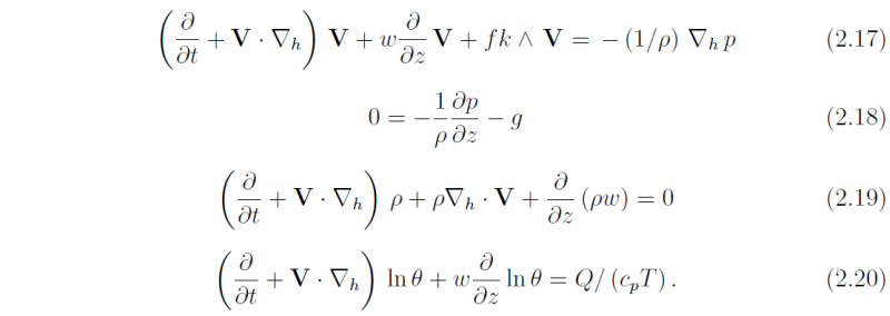
The basic equations for the motion of a dry atmosphere are.

 

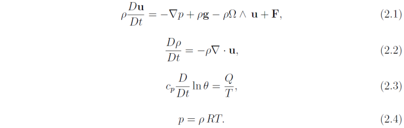
The first equation represents the conservation of momentum, the second the conservation of mass, the third the conservation of energy (first law of thermodynamics), and the fourth the equation of state. The variables u, p, ρ, T and θ and Q represent the (three-dimensional) fluid velocity, total pressure, density, temperature, potential temperature, and diabatic heating rate, respectively; F represents viscous and or turbulent stresses, and g is the effective gravity. The potential temperature is related to the temperature and pressure by the formula θ = T(p^*/p)^κ, where p^* = 1000 mb and κ = 0.2865.

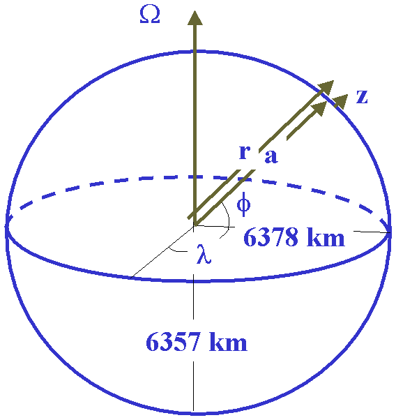
The shape of the �arth's surface is approximately an oblate spheroid with an equatorial radius of 6378 km and a polar radius of 6357 km. The surface is close to a geopotential surface, i.e. a surface which is perpendicular to the effective gravity (see DM, Chapter 3). As far as geometry is concerned the equations of motion can be expressed with sufficient accuracy in a spherical coordinate system (λ,φ,r), the components of which represent longitude, latitude and radial distance from the centre of the earth (see Fig. 1). The coordinate system rotates with the earth at an angular rate Ω = |Ω| = 7.292 × 10.5 rad s^-1.

An important dynamical requirement in the approximation to a sphere is that the effective gravity appears only in the radial equation of motion, i.e. we regard spherical surfaces as exact geopotentials so that the effective gravity has no equatorial component. Further details are found in Gill (1982; 4.12). Alternatively, the equations may be written in coordinates (λ,φ,z), where z is the height above the Earths surface (or more precisely the geopotential height). Note that r = a + z, where a is the earths radius. Since the atmosphere is very shallow compared with its radius (99% of the mass of the atmosphere lies below 30 km, whereas a = 6367 km), we may approximate r by a and replace ∂/∂r by ∂/∂z. In (λ,φ,z) coordinates, the frictionless forms of Eqs. (2.1) and (2.2) are (Holton, 1979, p 35):

 

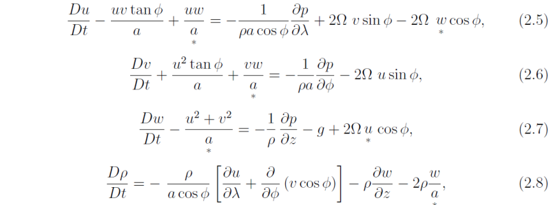
where u = a cos ��d�� dt i + r d�� dt j + dz dt k = ui + vj + wk. Here u, v and w represent the eastward, northward and vertical components of velocity, and D Dt �� �� ��t +u�E��, is the total-, or Lagrangian-, or material- derivative, following an air parcel. The terms with an asterisk beneath them will be referred to later.

2.2 The hydrostatic equation at low latitudes

In Chapter 1 we discussed the enormous diversity of motion scales which exists in low latitudes. We explore now the range of scales for which we may treat the motion as hydrostatic.

To carry out a scaling of (2.7) it is convenient to define a reference density and pressure, ρ₀(z) and p₀(z), characteristic of the tropical atmosphere and to define a perturbation pressure p' as the deviation of p from p₀(z). Then g in Eq. (2.7) must be replaced by the buoyancy force per unit mass, σ = -g(ρ - ρ₀(z))/ρ, and p may be replaced by p' in Eqs. (2.5) and (2.6). Details may be found in DM, Ch. 3. Omitting primes, (2.7) may be written

 

To perform the necessary scale analysis we let U, W, L, D, δp, Σ and τ represent typical horizontal and vertical velocity scales, horizontal and vertical length scales, a pressure deviation scale, a buoyancy scale and a time scale for the motion of a particular atmospheric system. The terms in (2.9) then have scales

 

For a value of δp = 1 mb (10² Pa) over the troposphere depth (20 km), δp/(ρD) ≈ 10² / (1.0 × 2.0 × 10⁴) = 0.5 × 10^-2 m s^-2. Also for U ≈ 10 m s^-1, Ω ≈ 10^-5 s^-1 and a ≈ 6 × 10⁶ m, the last two terms are of the order of 10^-4 and can be neglected.

The principal question is whether the vertical acceleration term can be neglected compared with the vertical pressure gradient per unit mass. To investigate this consider

We obtain an estimate for δp from the horizontal equation of motion (2.1). This yields two possible scales, depending on whether the motion is quasi-geostrophic, i.e. 1/ τ << f, or whether inertial effects predominate, 1/ τ >> f. In the latter case (fτ << 1),

 

while in the former case (1 << fτ)

 

If 1/τ = f, then, of course, δp ≈ P1 = P2. With the foregoing scales for P we can calculate the ratio in (2.11). Using P1 we find that

 

Thus in the high frequency limit (fτ << 1), hydrostatic balance will occur if W << U and/or D/L << 1, provided that the other ratio is no more than O(1). As we shall see later, this allows gravity waves to be treated hydrostatically, but the approximation is not valid for cumulus clouds.

In the low frequency limit (1 << fτ) we use P2, and obtain

 

Now, even if W ≈ U and D ≈ L, the hydrostatic approximation is justified provided 1 << fτ; which was the approximation that allowed us to obtain P anyhow. For synoptic-scale (L ≈ 10⁶), or planetary-scale (L ≈ a) motions, for both of which L >> D, the hydrostatic approximation is valid even if 1/τ ≈ f, and therefore as f decreases towards the equator. Thus we are well justified in treating planetary motions as hydrostatic.

We must be careful, however. We note that (2.5) has a component of the Coriolis force that is a maximum at the equator, i.e. although 2Ωvsinφ ← 0 as φ ← 0, 2Ωwcosφ ← 2Ωw. But in invoking the hydrostatic approximation we neglect the term 2Ωucosφ in (2.7). Thus forming the total kinetic energy equation with our new hydrostatic set we will produce an inconsistency. It appears in the following manner.

Multiplying (2.5) × u, (2.6) × v and (2.7) × w and adding, we obtain

We notice that all geometric terms and Coriolis terms have vanished by cancellation between the equations. This is as it should be as these terms are products of the geometry or are a consequence of Newtons second law being expressed in an accelerating frame of reference. That is, the terms would not appear as forces in an inertial frame and may not change the kinetic energy of the system. The problem is: if we make the assumption that the system is hydrostatic and note that for large scale flow, |w| << |u|, |v|, then the total kinetic energy may be written as

The last term in square brackets represents a fictitious or spurious energy source that arises from the lack of consistency in scaling the system of equations. Since each equation is interrelated to the others, it is incorrect to scale one without consideration of the others. Therefore, if the hydrostatic equation is used, energetic consistency requires that certain curvature and Coriolis terms must be omitted also. These are the terms marked underneath by a star in Eqs. (2.5) - (2.8). Similar considerations to these are necessary when "sound - proofing" the equations (see e.g. my advanced dynamical meteorology lectures ADM, Ch. 2).

The hydrostatic formulation of the momentum equations with friction terms included then becomes

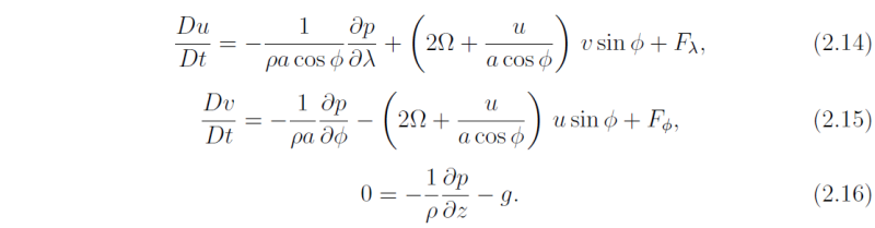
The need to neglect certain terms in the u and v equations to preserve energetic consistency has not been always appreciated. Many early numerical models, which were hydrostatic, could not conserve the total energy (i.e. kinetic and potential energy). The problem was traced to the inconsistency noted above.

2.3 Scaling at low latitudes

We consider now a more formal scaling of the hydrostatic equations in the vector form

Here V is the horizontal wind vector, w the vertical velocity component and ∇ is the horizontal gradient operator. We recognize that perturbations of pressure and density from the basic state p₀(z), ρ₀0(z) are relatively small, but seek to estimate their sizes for low- and middle-latitude scalings in terms of flow parameters.

We define a pressure height scale H_p such that 1/H_p = -(1/p₀)(dp₀/dz) and note that, using the hydrostatic equation for the basic reference state, H_p = p₀/(gρ₀). With the quasi-geostrophic scaling appropriate to middle-latitudes, Eq. (2.17) gives δp ≈ ρ₀fUL, whereupon

where Ro = U/fL is the Rossby number and Fr = U/√(gH) is a Froude number.

Note that (2.21) is satisfied even if Ro ≈ 1, because δp ≈ ρ₀fUL then provides the same scale as the inertial scale δp ≈ ρ₀U².

Hydrostatic balance expressed by (2.18) implies hydrostatic balance of the perturbation from the basic state, i.e. ∂p'/∂z = -gρ', whereupon it follows that δp/D ≈ gδρ, and therefore

assuming that D ≈ H_p.

Typically, g ≈ 10 m s^-2, Hp ≈ 10⁴ m whereupon, for U ≈ 10 m s^-1 f ≈ 10^-4 s^-1 (a middle-latitude value), Ro = 0.1 and F^-2 = 10³. It follows that in middle latitudes,

confirming that for geostrophic motions, fluctuations in p, ρ and θ may be treated as small.

At low latitudes, f ≈ 10^-5 s^-1 so that for the same scales of motion as above, Ro = 1. In this case, advection terms in (2.17) are comparable with the horizontal pressure gradient. However, as we have seen, the foregoing scalings remain valid for Ro ≈ 1 and therefore

Accordingly, we can expect fluctuations in p, ρ and θ to be an order of magnitude smaller in the tropics than in middle latitudes. The comparative smallness of the low-latitude perturbation may be associated with of the rapidity of the adjustment of the tropical motions to a pressure gradient imbalance; the adjustment being less constrained by rotational effects than at higher latitudes.

Consider now the adiabatic form of (2.20), i.e., put Q = 0. The scaling of this equation implies that

Using (2.23) and defining

where N is the buoyancy frequency and,

is a Richardson number, we have

an estimate that is valid for Ro = 1. It follows that, for the same scales of motion and in the absence of convective processes of substantial magnitude, we may expect the vertical velocity in the equatorial regions to be considerably smaller than in the middle latitudes. For example, for typical scales U = 10 m s^-1 , D = 10 km, L = 1000 km, Hp = 10 km, N = 10^-2 s^-1, Ri = 10² and W = 10^-3/Ro m s^-1. In the tropics, Ro ≈ 1 so that (2.26) would imply vertical velocities on the order of 10^-3 m s^-1, which is exceedingly tiny.

2.4 Diabatic effects, radiative cooling

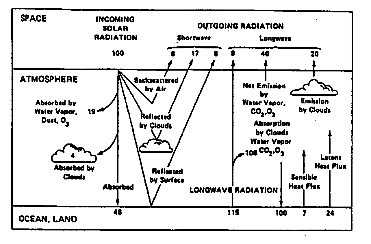
We shall see that in the tropics it is important to consider diabatic processes. We consider first the diabatic contribution in regions away from active convection so that the net diabatic heating is associated primarily with radiative cooling to space alone. Figure 2 shows the annual heat balance of the earths atmosphere. Of the 100 units of incoming short wave (SW) radiation, 31 units are reflected while the atmosphere radiates 69 units of long wave (LW) radiation to space. Accordingly, at the outer limits of the atmosphere, there exists radiative equilibrium. Altogether 46 units of SW radiation are absorbed at the surface. The surface emits 115 units of radiation in the long wave part of the spectrum, but 100 units of this are returned from the atmosphere. It is clear that, on average, there is a net radiative cooling of the atmosphere, amounting to 31 units, or 31% of the available incident radiation. 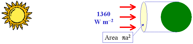On average, this cooling is balanced by a transfer of sensible heat (7 units) and latent heat (24 units) to the atmosphere from the earth's surface. The incoming solar radiation of 1360 W m^-2 (the solar constant) intercepted by the earth (πa² ≈ 1360 W) is distributed, when averaged over a day or longer, over an area 4πa² (see Fig. 3).

As discussed above, the atmosphere loses heat by radiation over 1 day or longer at the rate ΔQ = 0.31 × 0.25 × 1360 W m^-2. In unit time, this corresponds to a temperature change ΔT given by ΔQ = c_pMΔT, where M is the mass of a column of atmosphere 1 m^-2 in cross-section. Since M = (mean surface pressure)/g, we find that

Actually, the rate of cooling varies with latitude. From the surface to 150 mb (i.e. for ≈ 85% of the atmospheres mass), ΔT ≈ 1.2 K/day from 0^o - 30^o lat., -0.88 K/day from 30^o - 60^o3 lat., and -0.57 K/day from 60^o - 90^o lat. The stratosphere and mesosphere warm a little on average, but even together they have relatively little mass.

The estimate (2.25) suggests that for synoptic scale systems in the tropics, we can expect potential temperature changes associated with adiabatic changes of no more than a fraction of a degree. The estimate (2.26) shows that associated vertical motions are on the order of DU/(LRi), which is typically 10⁴ × 10/(10⁶ × (10^-4 × 10⁸/10²)) ≈ 10^-3 m s^-1.

In contrast, radiative cooling at the rate Q/cp = -1.2 K/day would lead to a subsidence rate which we estimated from (2.20) as

whereupon

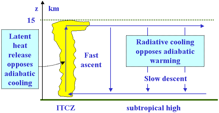
It follows that we may expect slow subsidence over much of the tropics and that the vertical velocities associated with radiative cooling are somewhat larger than those arising from synoptic-scale adiabatic motions.

We consider now the implications of the foregoing scaling on the vertical structure of the atmosphere. The vertical component of the vorticity equation corresponding with (2.17) and (2.18) is

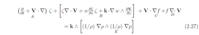
We compare the scales of each term in this equation with the scale for term A for Ro << 1 and Ro ≈ 1 (see Table 1).

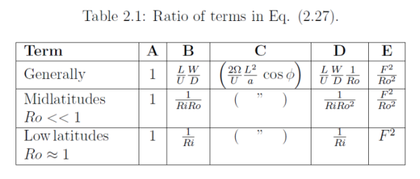
Using typical values chosen earlier (Ri = 10², F² = ) term C is O(1), while terms B, D and E are of order 10^-1, 1 and 10^-1 in the middle latitudes and of order 10^-2, 10^-2 and 10^-3 in the tropics, respectively. Thus, for Ro << 1, we have a general balance

whereas for Ro >= 1, the term D is reduced by more than two orders of magnitude and then

This is an important result. It tells us that outside regions where condensation processes are important, not only is the vertical velocity exceedingly small, the flow is almost barotropic. The implications are considerable. Such motions cannot generate kinetic energy from potential energy; they must obtain their energy either from barotropic processes such as lateral coupling or from barotropic instability.

We consider now the role of diabatic source terms. Again we assume that it is sufficient to approximate (2.20) by

but this time we assume that Q arises from precipitation in a disturbed region.

Budget studies have shown that three quarters of the radiative cooling of the tropical troposphere is balanced by latent heat release. From figures given earlier, this means for 0^o - 30^o lat., the warming rate is about 0.9 K/day. Gray (1973) estimated that tropical weather systems cover about 20% of the tropical belt. This would imply a warming rate Q/c_p ≈ 5 × 0.9 = 4.5 K/day in weather systems.

First let us calculate the rainfall that this implies. A rainfall rate of 1 cm/day (i.e. 10^-2 m/day) implies 10^-2 m³/day per unit area (i.e. m^-2) of vertical column. This would imply a latent heat release ΔQ ≈ LΔm per unit area per day, where L = 2.5 × 10⁶ J/kg is the latent heat of condensation and Δm is the mass of condensed water. Since the density of water is 10³ kg m^-3, we have ΔQ ≈ 2.5 × 10⁶ J/kg × 10^-2 m³ × 10³ kg/m³ per unit area = 2.5 × 10⁷ J/unit area/day. This is equivalent to a mean temperature rise δT in a column extending from the surface to 150 mb given by c_pm_aΔT ≈ 2.5 × 10⁷ J/unit area/day where m_a = (1000 - 150) mb/g is the mass of air unit area in the column. With c_p = 1005 J/K/kg we obtain ΔT ≈ 2.9.K/day.

Therefore, a heating rate of 0.9.K/day requires a rainfall of about 1/3 cm/ day averaged over the tropics, or 1.5 cm/day averaged over weather systems. Returning to (2.30) and, using the same parameters as before we find that a heating rate of 4.5 K/day leads to a vertical velocity of about 1.5 cm/sec, although the effective N² is smaller in regions of convection which would make the estimate for w a conservative one.

We can use these simple concepts to obtain an estimate for the horizontal area occupied by precipitating disturbances (see Fig. 3). Simply from mass conservation, the ratio of the area of ascent to descent must be inversely proportional to the ratio of the corresponding vertical velocities. Using the figures given above, this ratio is 1/3, but allowing for a smaller N in convective regions will decrease this somewhat, closer to Gray's estimate of 1/5.

2.5 Some further notes on the scaling at low latitudes

1. In mid-latitudes Ro << 1 and it is a convenient small parameter for asymptotic expansion. However, generally at low latitudes as f → 0, Ro ≈ 1 and we must seek other parameters. One such parameter, (RiRo)^-1 is always small, even if L ≈ 10⁷ m.

2. The vorticity equation contains useful information. It tells us that synoptic scale phenomena (L ≈ 10⁶ m) are nearly uncoupled in the vertical except in circumstances that limit (2.29). These are:

a. Q/c_p large. Then w is scaled from the thermodynamic equation such that wN²/g ≈ Q/(c_pT).

b. For planetary-scale motions (L ≈ 10⁷) of the type discussed in Chapter 1, we have again Ro << 1. Then, if D ≈ H_p as before, the quasi-geostrophic scaling (e.g., 2.24) applies once more. Moreover, the appropriate vorticity equation is (2.28) instead of (2.29). In this case, coupling in the vertical is re-established.

c. If the motions involve vertically-propagating gravity waves with D << H_p, but still with L ≈ 10⁷ m and if U → 0, then again Ro << 1 and vertical coupling occurs.

As a consequence of (2.29), the atmosphere is governed by barotropic processes. That is, the usual baroclinic way of producing kinetic energy from potential energy, i.e., the lifting of warm air and the lowering of cold air, does not occur. It follows then that energy transfers are strictly limited. How then can the kinetic energy be generated in the tropics? Obviously the answer lies in convective processes. But if this is so, why are the thermal fields so flat? This will be addressed later. However, it is interesting at this point to gain some insight into this feature of the tropical atmosphere.

If wN²/g ≈ Q/(c_pT), then < w'T' > ≈ g < Q'T' > /(N²c_pT). Now < w'T' > measures the rate of production of kinetic energy and g < Q'T' > is proportional to the rate of production of potential energy (i.e. heating where it is hot and cooling where it is cold). Thus the statement < w'T' > ≈ g < Q'T' > /(N²c_pT) implies that, in the tropics, potential energy is converted to kinetic energy as soon as it is generated. In other words there is no storage of potential energy. We know from scaling principles that wN²/g ≈ Q/(c_pT), as ∂θ/∂t and V • ∇ θ are relatively small in the tropics (see section 2.3). Since large precipitation implies large Q, it follows that w must be comparatively large as well.

If ∇T were large, a third term would enter such that < w'T' > +(g/N²) < T'V' > • ∇T ≈ < Q'T' >/(c_pT) and this is tantamount to having storage even if V is the same in both cases.

2.6 The weak temperature gradient approximation

One can derive a balanced theory for motions in the deep tropics by assuming that ∂θ/∂t and V • ∇ θ are much less than w(∂θ/∂z), whereupon

where S_θ = Q/(c_pπ), π = (p/po)^κ is the Exner function, and p_o = 1000 mb. The vorticity equation (2.28) may be written

where D is the horizontal divergence ∇ • V, and the continuity equation gives

Using (2.31) the vorticity equation becomes

If there were no diabatic heating (S_θ = 0), the right-hand-side of (2.33) would be zero and absolute vorticity values would be simply advected around at fixed elevation by the horizontal wind. The role of heating is to produce vertical divergence, which, in turn, decreases the absolute vorticity if the divergence is positive and increases it if the divergence is negative (i.e. if there is horizontal convergence). If the divergence and the horizontal wind fields are known, it is therefore possible to predict the evolution of the absolute vorticity field.

The final difficulty is predicting the horizontal wind field. The horizontal wind components can be written as sums of parts derived from a streamfunction φ and parts derived from a velocity potential χ

However, φ and χ may be written in terms of ζ_a and D:

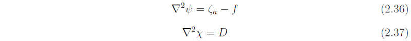
where ∇² is the horizontal Laplacian operator. Equations (2.36) and (2.37) are readily solved for ψ and χ using standard numerical methods, after which the horizontal velocity may be determined from (2.35). Given the horizontal velocity and the divergence, we have the tools needed to completely solve the vorticity equation. In practice, (2.34), stepped forward in time and the diagnostic equations (2.36) and (2.37) are solved after each time step to enable the velocity field to be updated using (2.35). All that is required to close the system is a method of specifying the heating term S_θ.

The principal determinant of the sign of the horizontal divergence in (2.33) is the sign of ∂S_θ/∂z. If heating increases with height, divergence is negative, and the magnitude of the absolute vorticity increases with time, whereas S_θ decreasing with height results in positive divergence and decreasing absolute vorticity. Deep convection generally results in increasing vorticity or spinup in the lower troposphere and spindown in the upper troposphere, whereas other regions typically dominated by radiative cooling and shallow convection tend to experience the reverse.

In spite of the fact that tropical storms don't formally obey the weak temperature gradient approximation, the above picture holds qualitatively for them as well. However, gravity wave dynamics are not encompassed by this picture, so the wind perturbations associated with these waves are not captured. Furthermore, consideration of frictional effects is important to the quantitative prediction of tropical flows, especially in the long term. In spite of these deficiencies, the above picture of tropical dynamics should be useful for understanding the short-term evolution of most tropical weather systems. In a later chapter we approach the problem of determining the pattern of heating associated with moist convection. More details on the weak temperature gradient approximation can be found in papers by Sobel and Bretherton (2000), Sobel et al. (2001) and Raymond and Sobel (2001).

Copyright © Roger Smith, Date 10 Apr 2015