User Tools
Sidebar
Table of Contents
Case C 2: Cubic cloud
Setup:
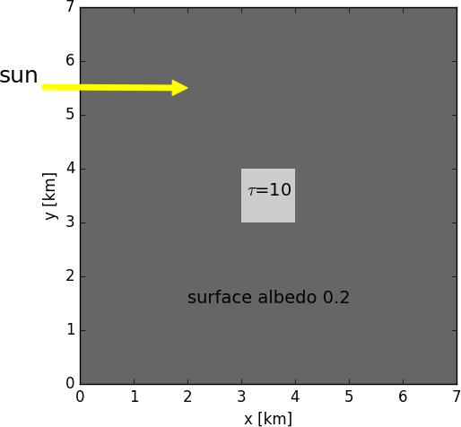
- simple cubic cloud
- domain: 7×7 km$^2$ in x-y-plane, 5 km in z direction
- cubic cloud 1x1x1 km$^3$ in domain center: x: 3-4km, y: 3-4km, z: 2-3km
- 70×70 pixels along x-y direction
- periodic boundary conditions
- vertical optical thickness of cloud: 10
- homogeneous extinction coefficient in cube
- optical properties as for case C 1 (step cloud)
- single scattering albedo: 1.0
- effective radius: 10 $\mu$m
- Lambertian surface albedo: 0.2
- Solar azimuth angle $\phi_0$=0$^\circ$
- Viewing geometries (solar zenith angle $\theta_0$, output altitude $z$, viewing zenith angle $\theta$ and viewing azimuth angle $\phi$):
| # | $\theta_0$ [$^\circ$] | $z$ [km] | $\theta$ [$^\circ$] | $\phi$ [$^\circ$] |
|---|---|---|---|---|
| 1 | 20 | 0 | 40 | 0 |
| 2 | 20 | 0 | 40 | 60 |
| 3 | 20 | 0 | 40 | 120 |
| 4 | 20 | 0 | 40 | 180 |
| 5 | 40 | 5 | 180 | 0 |
| 6 | 40 | 5 | 140 | 0 |
| 7 | 40 | 5 | 140 | 60 |
| 8 | 40 | 5 | 140 | 120 |
| 9 | 40 | 5 | 140 | 180 |
- first set of simulations: cubic cloud in vacuum
- second set of simulations: cubic cloud in homogeneous Rayleigh scattering layer with optical thickness of 0.5, depolarization factor 0
Note on azimuth convention:
                            270
                   +++++++++++++++++high Y
                   |                     |
                   |                     |
                   |                     |
            0 deg  |                     | 180
                   |                     |
                   |                     |
                   ++++++++++++++++++low Y
                            90
                   low X            high X
Output format:
The output should be provided in an ascii file containing the following columns:
case theta_0 z theta phi i_x i_y I Q U V Istd Qstd Ustd Vstd
case should be set to 1 for the simulations in vacuum and 2 for the case with Rayleigh scattering.
i_x and i_y denotes the pixel numbers in x and y direction respectively (starting with 1).
I,Q,U,V denote the Stokes vector.
Istd Qstd Ustd Vstd are standard deviations of the Stokes vector components which should be provided for Monte Carlo models. If error estimates can not be provided, these columns may be omitted.
The result filename should be 'iprt_case_C2_MODEL.dat' and it should include the following header:
# IPRT case C2 - Cubic cloud
# RT model: MODEL_NAME
# case theta_0 z theta phi i_x i_y I Q U V Istd Qstd Ustd Vstd
Data of model results
Results without atmosphere
Plots of MYSTIC results
The following plots show the results obtained with MYSTIC. For all other models the patterns look the same.
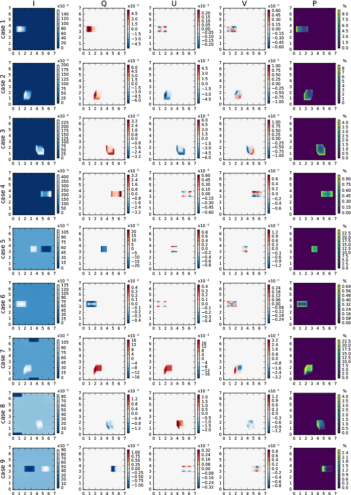
General remarks:
- Generally we find a very good agreement between all Monte Carlo models
- The polarization patterns are the same in all models, also the pattern for V when variance reduction methods are applied
- For SHDOM a quantitative comparison is difficult because it does not provide a standard deviation and systematic differences are expected (different treatment of cloud boundary, smaller differences due to different solution method of VRTE).
- MSCART (backward mode) shows systematic differences to the forward calculations, Wang Zhen already mentioned this. MYSTIC gives the same results in forward and backward mode.
- The agreed number of photons for this case is 49e9, this number has been used for 3DMCPOL, MSCART and MYSTIC. For SPARTA, 1e11 photons were used
- Circular polarization (Stokes component V) is very noisy in Monte Carlo results, especially for models without variance reduction.
Statistics of model intercomparison
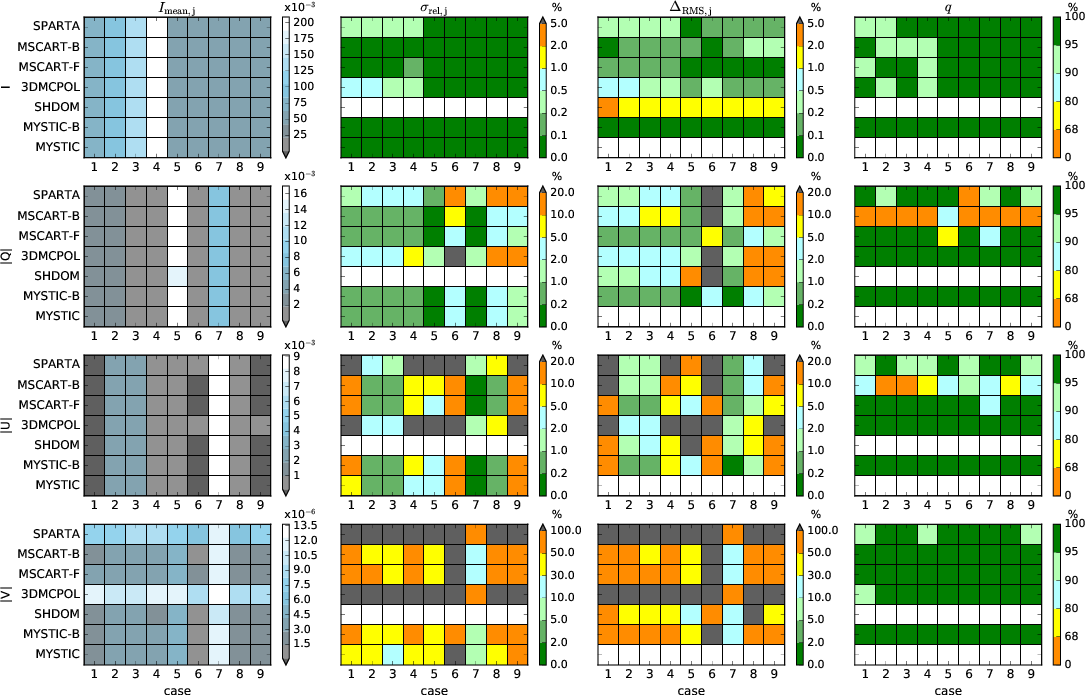 Statistics of the Stokes vector results for scenario C2 (cubic cloud
in vacuum). The panels in the left column show the mean radiance
$I_{\rm mean}$ (for Q, U, and V the mean of the absolute values) for
all models and all 9 cases. The panels in the second column show the
standard deviations $\sigma_{\rm rel}$. The third column shows the
root mean square differences $\Delta_{\rm RMS}$ with respect to MYSTIC
in per cent and the right column shows the match fractions $q$.
Notes:
- Stokes component I: The mean radiance (average over all non-zero pixels) is very similar for all models. The RMS difference is < 1% for all MC models, <1.5% for SHDOM. Standard deviations are much smaller when variance reduction techniques are used (as expected).
The match fraction shows that all Monte Carlo models agree within 2σ for cases 5-9 (down-looking). The match fraction is between 0.9 and 0.95 for some up-looking cases 1-4, which might indicate a small bias between other models and MYSTIC. However, the number of non-zero pixels included in the statistics is only 200, so that values between 0.9 and 0.95 are still ok. - Stokes component Q (second row): The first column shows the mean absolute radiance (since Q can be positive or negative). \\Mean standard deviations again are larger for models without variance reduction. The match fraction shows obvious systematic differences for mscart_bmc (all cases), mscart_fmc (cases 5 and 7) and SPARTA (case 6). RMS difference for mscart case 1 looks too large, CE will check this.
- Stokes component U (third row): The match fraction shows obvious systematic differences for mscart_bmc (all cases), mscart_fmc (case 7).
- Stokes component V (bottom): Very noisy, without variance reduction (SPARTA, 3DMCPOL) noise is much larger than mean radiance. The match fraction shows systematic differences for mscart_bmc and mscart_fmc (all cases). These differences might be numerical because the mean radiance is very small (about 2e-6). Since the standard deviation is an order of magnitude larger than the radiance for SPARTA and 3DMCPOL, the results mostly match within 2σ, but this does not show whether the models really agree.
- Generally the standard deviation for SPARTA is below 3DMCPOL because for SPARTA more photons were used (10e11 vs. 49e9). MYSTIC and MSCART used 49e9 photons and variance reduction techniques which decrease the standard deviation approximately by almost one order of magnitude.
- RMS differences should only be looked at when mean radiance value is not too small (>1e-3). Here it is genearally <5% for Q and U for all cases and all models. For I it is <1%.
Results with atmosphere
Plots of MYSTIC results with atmosphere
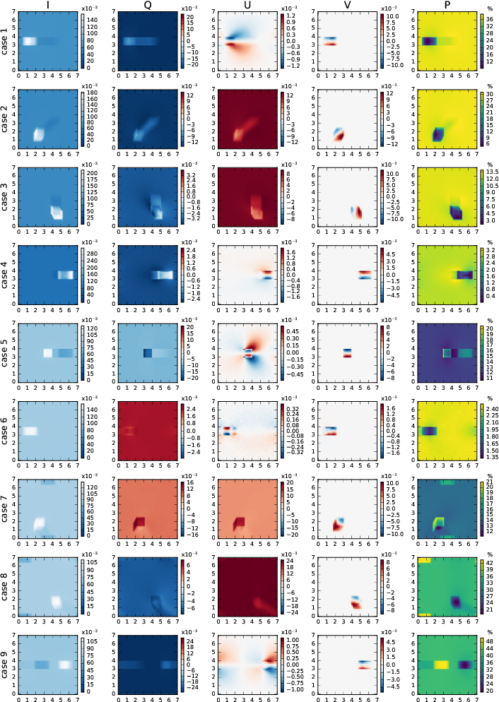
The following plots show the results obtained with MYSTIC. As for the cases without atmosphere the patterns look the same for all models.
Statistics of model intercomparison
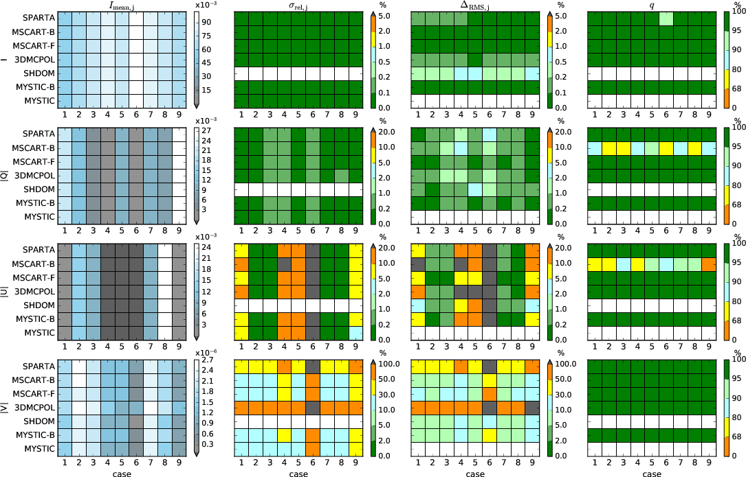 Statistics of the Stokes vector results for scenario C2 (cubic cloud
in vacuum). The panels in the left column show the mean radiance
$I_{\rm mean}$ (for Q, U, and V the mean of the absolute values) for
all models and all 9 cases. The panels in the second column show the
standard deviations $\sigma_{\rm rel}$. The third column shows the
root mean square differences $\Delta_{\rm RMS}$ with respect to MYSTIC
in per cent and the right column shows the match fractions $q$.
Notes:
- Stokes component I (upper row): Mean radiance agrees very well for all models. The mean standard deviations are in the range from 2e-5 to 5e-5, here the difference between models with variance reduction and without is not as large as for the cases without atmosphere. The reason is that for cases with atmosphere, there are no pixels with zero radiance and all pixels are now included in the statistics. In the clearsky region the standard deviation is not reduced by variance reduction. The match fraction shows a perfect agreement between all Monte Carlo codes over the full image.
- Stokes component Q (second row): Mean absolute radiance agrees well for all models. As for I the standard deviations are similar for all codes. The match fraction shows a perfect agreement between all Monte Carlo codes, except MSCART (backward mode). MYSTIC (backward mode) agrees perfectly to MYSTIC run in forward mode.
- Stokes component U (third row): Mean absolute radiance agrees well. Match fraction again shows perfect agreement for all Monte Carlo codes except MSCART (backward mode).
- Stokes component V (fourth row): Mean radiances agree within noise. Largest differences (still below 5e-6) for MSCART. Standard deviation is significantly reduced by variance reduction, because V is only non-zero in cloud (only cloud scattering causes circular polarization, molecular scattering does not). Pixels with zero V are not included in statistics, thus standard deviation is more influenced by variance reduction. Very small systematic differences (may be numerical) between MYSTIC and MSCART (forward and backward).
- Standard deviations are smaller in forward than in backward mode, when the same number of photons/pixel (i.e. 1e7) is used. This can be seen for MYSTIC and also for MSCART.
- RMS mostly for I<1%, for Q and U<2% (for mean Q,U > ~1e-3) and for V <20% (for models with variance reduction and SHDOM).
Detailed plots for all models, no atmosphere
Statistics plots
Stokes parameters I,Q,U,V
Differences to MYSTIC
Detailed plots for all models - with atmosphere
Statistics plots
Stokes parameters I,Q,U,V
The range of the colorbars corresponds to the minimum and the maximum of the SHDOM results. For V all Monte Carlo models show quite strong noise, therefore the best is to choose the explicit model to set the limits.
Differences to MYSTIC
Here the colorbar limits correspond to 5% of the minimum and maximum of the MYSTIC results.

