intercomparisons:c3

Case C3: Cumulus cloud
Data of model results
Results for pure Rayleigh background atmosphere
Results with atmosphere
Detailed plots for all models, pure molecular atmosphere
Detailed plots for all models - molecular atmosphere including aerosol

Case C3: Cumulus cloud

Setup:

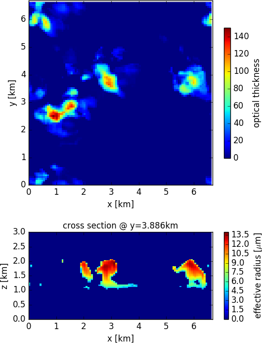
Cumulus cloud field from LES model (same as used in I3RC project, $r_{\rm eff}$ depending on LWC):

cumulus.dat, the format of the ascii file is as follows:

    Nx Ny Nz flag
    dx dy z1 z2 z3 .... 
    ix iy iz ext Reff
      ...

The number of horizontal pixels is Nx x Ny = 100×100 in the horizontal and Nz=53 in the vertical. The horizontal resolution is dx x dy = 0.0667km x 0.0667km, hence the domain size is 6.67×6.67 km$^2$. The 54 vertical layer grid points are specified by z1, z2, … zn, the grid is not equidistant. The file includes the extinction coefficient ext [km$^{-1}$] and the effective radius Reff [$\mu$m] for cloudy grid cells. Cloudfree grid cells are not included in the file. The grid cell is specified by indices ix, iy, iz (each starting with 1).

output radiances are requested on the same grid (100×100 pixels).
periodic boundary conditions
Cloud optical properties from Mie calculations (same information in netcdf and ascii file): watercloud_670.mie.cdf
Aerosol optical properties for the same aerosol type as used for case A3 (same information in netcdf and ascii file): waso_670.mie.cdf, waso_670.mie.dat
Layer optical thicknesses of model atmosphere: atmos_tau_cu.dat (file includes profiles for molecular absorption, Rayleigh scattering and aerosol extinction)
Same information for model levels (extinction coefficients): atmos_ext_cu.dat
Rayleigh depolarization factor: 0
wavelengths: 670 nm
Lambertian surface albedo: 0.2
Solar azimuth angle $\phi_0$=0$^\circ$
Viewing geometries (solar zenith angle $\theta_0$, output altitude $z$, viewing zenith angle $\theta$ and viewing azimuth angle $\phi$), same as for C2:

#	$\theta_0$ [$^\circ$]	$z$ [km]	$\theta$ [$^\circ$]	$\phi$ [$^\circ$]
1	20	0	40	0
2	20	0	40	60
3	20	0	40	120
4	20	0	40	180
5	40	30	180	0
6	40	30	140	0
7	40	30	140	60
8	40	30	140	120
9	40	30	140	180

first set of simulations: cloud field and molecular atmosphere (both molecular absorption and Rayleigh scattering)
second set of simulations: cloud field, molecular atmosphere, and aerosol profile

Note on azimuth convention: (This is taken from the I3RC definition)

                            270
                   ++++++++++++++++++high Y
                   |                     |
                   |                     |
                   |                     |
            0 deg  |                     | 180
                   |                     |
                   |                     |
                   ++++++++++++++++++low Y 
                            90
                   low X            high X

Output format:

The output should be provided in an ascii file containing the following columns:

case  theta_0  z  theta  phi  i_x i_y I  Q  U  V  Istd  Qstd  Ustd  Vstd

case should be set to 1 for the simulations with Rayleigh scattering and to 2 for the simulation with aerosol.

i_x and i_y denotes the pixel numbers in x and y direction respectively (starting with 1).

I,Q,U,V denote the Stokes vector.

Istd Qstd Ustd Vstd are standard deviations of the Stokes vector components which should be provided for Monte Carlo models. If error estimates can not be provided, these columns may be omitted.

The result filename should be 'iprt_case_C2_MODEL.dat' and it should include the following header:

# IPRT case C3 - Cumulus cloud 
# RT model: MODEL_NAME 
# case theta_0 z theta phi i_x i_y I Q U V Istd Qstd Ustd Vstd

Data of model results

Results of MYSTIC model.

Results of all models (MYSTIC, SHDOM, SPARTA, 3DMCPOL, MSCART).

Results for pure Rayleigh background atmosphere

MYSTIC results

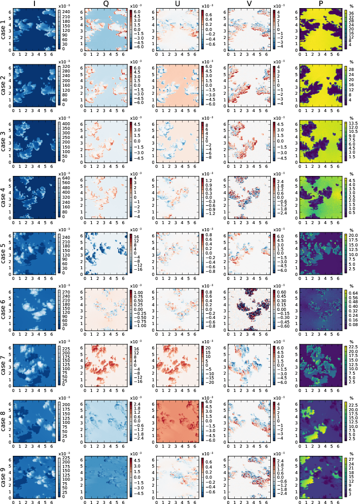
The following plots show the results obtained with MYSTIC. For all other models the patterns look the same.

General remarks

Generally we find a very good agreement between all Monte Carlo models
The polarization patterns are the same in all models, also the pattern for V when variance reduction methods are applied
For SHDOM a quantitative comparison is difficult because it does not provide a standard deviation and systematic differences are expected (different treatment of cloud boundary. Smaller differences due to different solution method of VRTE).
The agreed number of photons for this case is 10e10 (1e6 photons per pixel), this number has been used for all Monte Carlo models (3DMCPOL, MSCART, SPARTA and MYSTIC)
Circular polarization (Stokes component V) is very noisy in Monte Carlo results.

Statistics

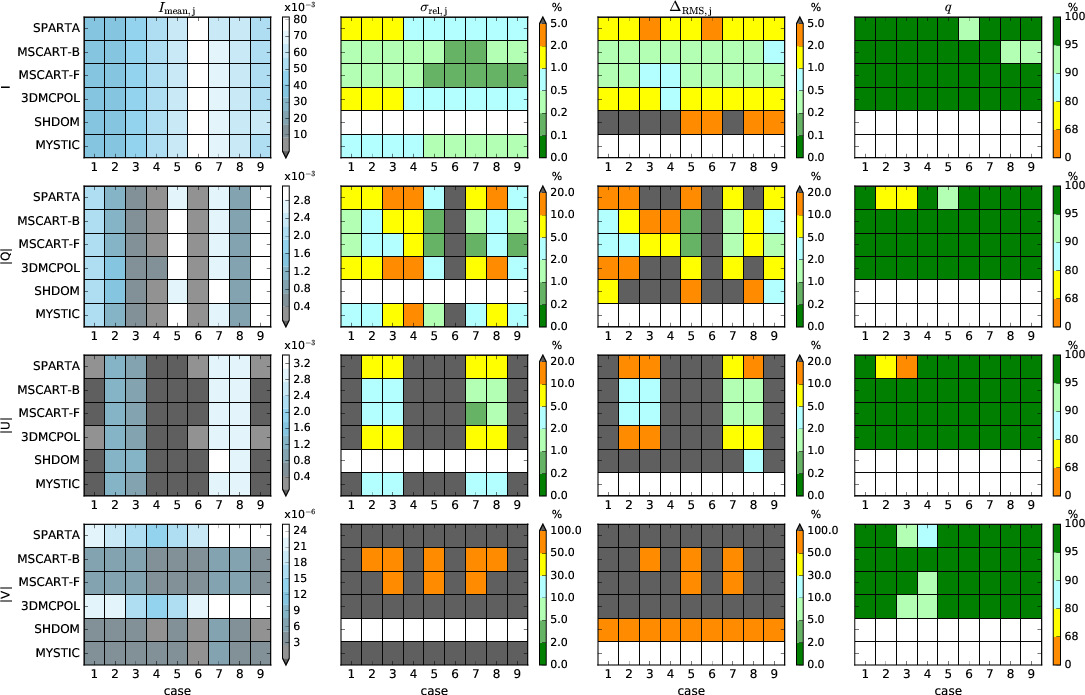Statistics of the Stokes vector results for scenario C3 (cumulus cloud field in molecular atmosphere). The panels in the left column show the mean radiance $I_{\rm mean}$ (for Q, U, and V the mean of the absolute values) for all models and all 9 cases. The panels in the second column show the standard deviations $\sigma_{\rm rel}$. The third column shows the root mean square differences $\Delta_{\rm RMS}$ in per cent and the right column shows the match fractions $q$.

Notes:

Stokes component I (upper row): Obvious differences in mean radiances only for SHDOM. The mean standard deviation is almost the same for 3DMCPOL and SPARTA, both models use the same number of photons and no variance reduction. The standard deviation of MSCART is smallest, so for this case it seems that MSCART variance reduction works best. The match fraction shows that all Monte Carlo codes agree.
Stokes component Q (second row): Results are similar to I, however we find systematic differences for SPARTA (cases 2 and 3)
Stokes component U (third row): Also for U, there are systematic differences between SPARTA and other Monte Carlo models for cases 2 and 3.
Stokes component V (bottom row): Mean radiance for V is dominated by noise, so here we can not compare the models quantitatively.

Results with atmosphere

MYSTIC results

The following plots show the results obtained with MYSTIC. As for the cases without atmosphere the patterns look the same for all models.

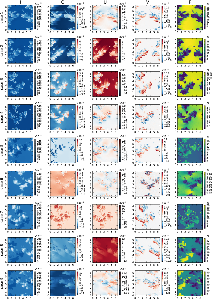
Statistics

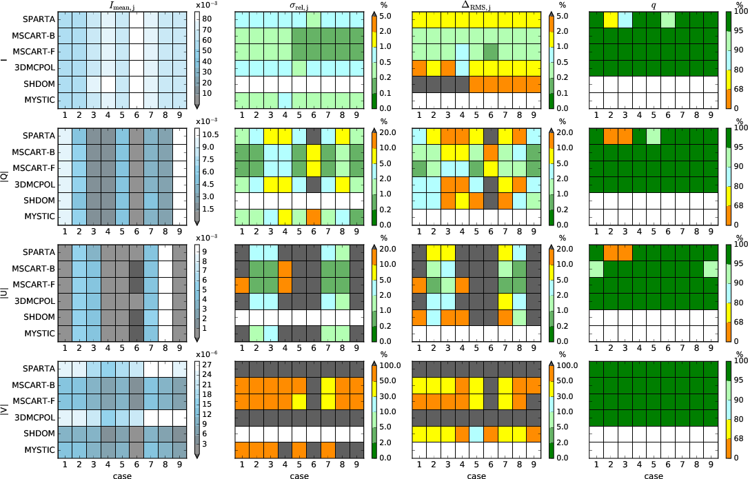Statistics of the Stokes vector results for scenario C3 (cumulus cloud field and aerosol in molecular atmosphere). The panels in the left column show the mean radiance $I_{\rm mean}$ (for Q, U, and V the mean of the absolute values) for all models and all 9 cases. The panels in the second column show the standard deviations $\sigma_{\rm rel}$. The third column shows the root mean square differences $\Delta_{\rm RMS}$ in per cent and the right column shows the match fractions $q$.

Notes:

Stokes component I (upper row): Mean radiances agree well, largest differences for SHDOM. Match fraction shows systematic differences for SPARTA, again cases 2 and 3 as for case without aerosol. MSCART variance reduction more efficient than MYSTIC.
Stokes components Q and U: Similar results as for I.
Stokes component V: Results dominated by noise, no quantitative comparison possible.

Detailed plots for all models, pure molecular atmosphere

Statistics plots

Stokes parameters I,Q,U,V

Differences to MYSTIC

Detailed plots for all models - molecular atmosphere including aerosol

Statistics plots

Stokes parameters I,Q,U,V

The range of the colorbars corresponds to the minimum and the maximum of the SHDOM results. For V all Monte Carlo models show quite strong noise, therefore the best is to choose the explicit model to set the limits.

Differences to MYSTIC

Here the colorbar limits correspond to 5% of the minimum and maximum of the MYSTIC results.