Mie phase function at 500 nm for an effective droplet size of 10 μm.

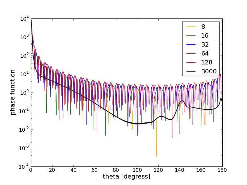
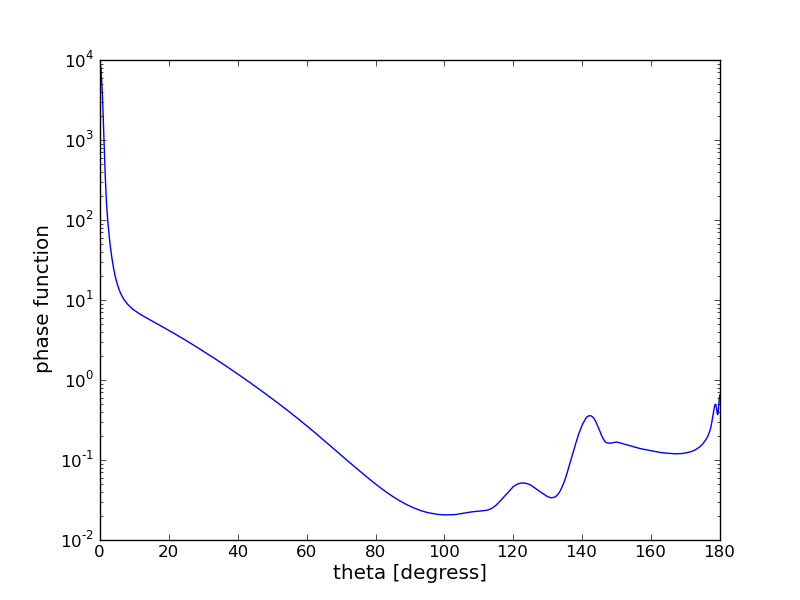
Task: The file phase_function_500nm_reff10.dat includes a typical scattering phase function for cloud water droplets. It has been computed using Mie theory (mie tool in libRadtran). In order to apply the discrete ordinate method the phase function is expanded in a Legendre series. The number of terms in the Legendre series is equal to the number of streams (nstr). Investigate how many Legendre terms are required to represent the phase function as a Legendre series.

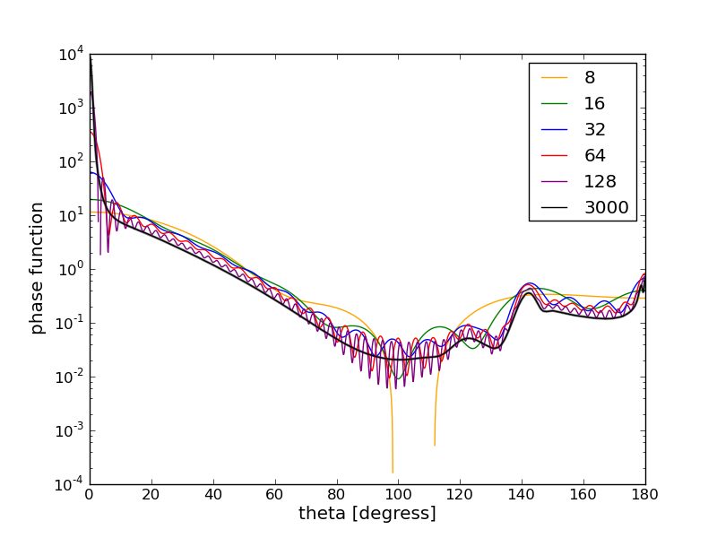
The so-called delta scaling method (see wiscombe77b.pdf) is used to represent the phase function with less number of Legendre terms by writing it as a sum of a delta function (representing the forward scattering peak) and a Legendre series for a phase function with cutted forward scattering peak. Explain the delta scaling method and check how much improvement can be achieved using this method.

LibRadtran includes 2 tools which can be used for this task:

pmom - calculates Legendre polynomials for given phase function

phase - calculates phase function for given Legendre polynomials (with or without delta scaling)

Both tools are in the libRadtran/bin directory and help is obtained using the option -h.

The following shell script calculates Legendre polynomials and the phase functions corresponding to different number of terms in the Legendre series:

gen_legendre.sh

 # Expand phase function in Legendre polynomials
for i in 4 8 16 32 64 128 3000; do pmom -l $i -n phase_function_500nm_reff10.dat > nmom$i.dat; done
 
# Calulate phase function from Legendre polynomials
for i in 4 8 16 32 64 128 3000; do phase -c -d -s 0.1 nmom$i.dat > phase$i.dat; done
 
# Calulate phase function from Legendre polynomials with delta scaling
for i in 4 8 16 32 64 128 3000; do phase -c -d -s 0.1 -f nmom$i.dat > phase$i\_ds.dat; done

The shell script is executed as follows:

   sh gen_legendre.sh

The result is plotted using the following python scipt

plot_legendre.py

   from pylab import *
 
colors=['orange', 'g', 'b', 'r', 'purple', 'k']
 
phase_orig=loadtxt('phase_function_500nm_reff10.dat')
 
figure(1)
semilogy(phase_orig[:,0], phase_orig[:,1], 'grey', lw=2)
 
figure(2)
semilogy(phase_orig[:,0], phase_orig[:,1], 'grey', lw=2)
 
i=0
for nmom in ['8', '16', '32', '64', '128', '3000']: 
 
    figure(1)
    phase=loadtxt('phase'+nmom+'.dat')
    semilogy(phase[:,0], phase[:,1], colors[i], label=nmom)
    xlabel('theta [degress]')
    ylabel('phase function')
 
    figure(2)
    phase=loadtxt('phase'+nmom+'_ds.dat')
    semilogy(phase[:,0], phase[:,1], colors[i], label=nmom)
    xlabel('theta [degress]')
    ylabel('phase function')
 
    i+=1
 
figure(1)
legend()
savefig('phase_without_ds.png')
 
figure(2)
legend()
savefig('phase_with_ds.png')

With delta scaling the approximation of the phase function becomes much better. Note that the forward scattering peak is reduced by delta-scaling, the smaller the number of terms in the Legendre series the more. Already for 16 termns there are no very strong oszillations including negative values so that DISORT2 should calculate reasonable (not so accurate) radiances.

DISORT2 includes an intensity correction method (which uses the correct phase functions for two orders of scattering). This gives then very accurate radiance results.