Effective emission of thermal radiation of a single layer

I recently changed the emission of thermal radiation. It used to be the planck emission of the mean temperature of a layer and use that in all directions, i.e. upward and downward emission have been the same.

To be more consistent with DISORT and RRTMG calculations I opted to change that in favor of a linear interpolation of level temperatures. In the following graph we see the effective emissions of a single layer depending on the optical depth and various methods. $B_2$ denotes the interface which is further away, $B_1$ is the interface at which we are interested in the emission value.

First the old implementation used the emission due to a mean temperature $B(T_{mean})$. Subsequently, the first thing I tried was to interpolate it with the emissivity of diffuse transmission coefficient, $a_{11}, a_{a12}$ for that matter):

$$B_{eff,2str} = B1 * \int_0^1 e^{-\tau/\mu}\ d\mu + B2 * (1 - \int_0^1 e^{-\tau/\mu}\ d\mu)$$

This is the purple line in the below graph. It quickly became obviuous that this was a bad idea…

Bernhard did an analytical computation with the linear interpolation ansatz:

$$B(\tau) = B_1 + (B_2 - B_1) \frac{\tau}{\tau_0}$$

where $\tau_0$ is the vertical optical depth. If we plug that into the schwarzschild ansatz:

$$\mu \frac{dL}{d\tau} = B -L = B1 + (B2 - B1) \tau - L$$

we end up with a solution as:

$$L(\tau) = \frac{(-B_1 + \frac{B_2-B_1}{\frac{\tau}{\mu}}) e^\frac{-\tau}{\mu} + B_1 + \frac{B_2-B_1}{\tau} (\tau - \mu)}{1-e^\frac{-\tau}{\mu} }$$

Further, resubstituting with

$$L(\tau) = B_{eff} (1-e^\frac{\tau}{\mu})$$

gives:

$$B_{eff}(\tau) = \frac{(-B_1 + \frac{B_2-B_1}{\frac{\tau}{\mu}}) e^\frac{-\tau}{\mu} + B_1 + \frac{B_2-B_1}{\tau} (\tau - \mu)}{1-e^\frac{-\tau}{\mu} }$$

The expression can be simplified to:

$$B_{eff}(\tau) = \frac{ B_2 e^\frac{-\tau}{\mu} - B_1 } { e^\frac{-\tau}{\mu} - 1 } + \frac{B_2 - B_1}{\frac{\tau}{\mu}}$$

which is also given in the below plot, for varying angles $\mu=1$, $\mu=.5$, and integrated over the halfspace.

Finally, I also computed the thermal emission via a schwarzschild approach with the following code:

# Explicit numeric solution
def schwarzschild_tau(T1, T2, tau=1., Nmu=100):
    Nlay = 1000
    dtau = tau/Nlay
    Tlev = linspace(T1,T2,Nlay+1)
    Blay = B( (Tlev[1:]+Tlev[:-1])/2 ) / pi
    dmu = 1./Nmu

    B_eff= 0
    for mu in arange(dmu/2,1.,dmu):
        L = 0 # lower bound
        t = exp(-dtau/mu) # transmission
        for k in range(Nlay):
            L = L * t + (1.-t) * Blay[k] # extinction plus emission with mean temperature
        B_eff += L * mu * dmu

    return B_eff * 2*pi

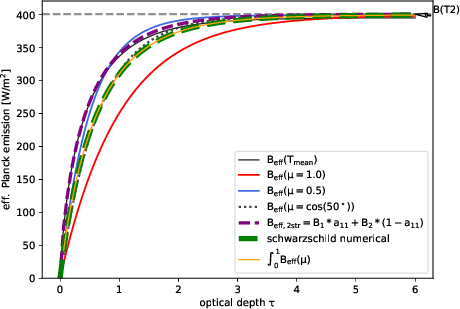
Or look at the effective emission value without the respective emissivity: 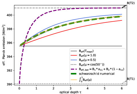The various lines are:

$B_{eff}(T_{mean})$ just using the mean temperature
$B_{eff}(\mu=1)$ using above stated analytic function with $\mu=1$
$B_{eff}(\mu=.5)$ … with $\mu=0.5$
$B_{eff}(\mu=cos(50^\circ))$ with $\mu=0.6427$ which is the $\mu$ that minimizes the error up to $\tau=100$
$B_{eff,2str}$ using the integral formulation from the first step with the twostream coefficients
schwarzschild numerical subdivides the layer into 1000 thin layers to get $\tau << 1$
$\int_{0}^{1} \rm B_{eff}(\mu)$ integrates the above analytic function on legendre quadrature points

Conclusions:

It is clear that the old way of using the mean temperature planck emission(black line) gives comparable results as the approach with the transmission weighted formulation and both of them fail for opticallyt thin layers. Furthermore we note that Bernhards analytic formulation gives the same results as the numerical integration in the schwarzschild fashion however we cannot find a single representative value for $\mu$ that works for all optical thicknesses. I tried to integrate the analytic version over $\mu$ but didnt come up with a good solution, hence in the Tenstream, I integrate it with legendre quadrature points (see src/schwarzschild.F90::B_eff()).

Code:

The full code for the plot can be found … here