As discussed in Chapter 2, tropical cyclones originate from convective cloud systems and a distinguishing feature of the mature tropical cyclone is the ring of deep clouds that form the eyewall and the largely cloud-free eye. In this chapter we review of basic concepts necessary to understand moist convection. In the following chapter we explore the role of moist convection in the dynamics of tropical cyclone intensification, focussing on the collective effects of clouds in an axisymmetric framework. We begin here with a brief discussion of convective instability and go on to examine three types of convection: shallow convection, which as the name suggests has a limited vertical extent, and deep convection, which extends through much or all of the troposphere and intermediate convection, where the cloud tops remain below the freezing level, which is about 5.5 km in the tropics.
The occurrence of moist convection in the atmosphere is frequently explained in terms the behaviour of an ascending air parcel that does not mix with its environment. When an unsaturated air parcel is lifted adiabatically, it expands and and cools. Since the maximum amount of water vapour it can hold decreases strongly as its temperature decreases, it eventually reaches a level at which it becomes saturated. This is the so-called lifting condensation level, or LCL. If the parcel is lifted above this level, water progressively condenses and the latent heat that is released reduces the rate at which the parcel cools. Typically a parcel is still denser than its environment at the LCL and is therefore negatively buoyant. However, if the lifting continues, it may reach a level at which it becomes lighter than its environment and therefore positively buoyant. This level is called the level of free convection (LFC). Above this level the parcel can accelerate under its own buoyancy force until at some further level it again becomes neutrally buoyant. This level is called the level of neutral buoyancy, or LNB. Above the LNB the parcel has negative buoyancy and usually rapidly decelerates. The various levels described above are usually estimated on the basis of an aerological diagram, which is a judiciously transformed thermodynamic diagram. In its most basic form, a thermodynamic diagram is one in which the pressure and specific volume are plotted on the ordinate and abscissa, respectively. Then according to the equation of state (1.9), the isotherms are rectanglar hyperbolae. The state of a parcel of dry air can be represented by a point in such a diagram and the change in state as the pressure and specific volume change can be represented as a curve. For example, an isothermal change is represented by a rectangular hyperbola. The p-\alpha-diagram is of limited practical use in meteorology because the specific volume is not a quantity that is measured. An aerological diagram is transformed version in which more relevant meteorological variables are displayed and lines representing state changes associated with important atmospheric processes are plotted. There are various kinds of such diagrams, one being the tephigram and another the skew-T log-p diagram. In this diagram the isobars are straight horizontal lines and are plotted with a logarithmic scale with pressure decreasing upwards so that the ordinate is approximately equal to height. The isotherms are straigt lines that run upwards to the right at an angle of 45 degrees. Also plotted are the dri-adiabats, curves curves on which the potential temperature is constant; the moist adiabats, curves on which the pseudo-equivalent potential temperature is constant; and curves of constant saturation mixing ratio. While the state of a sample of dry air is represented by a single point in the diagram, that of a moist sample requires two points, one corresponding to the pressure and temperature of the parcel and the second corresponding to the pressure and dew-point temperature, Td. The saturation mixing ratio line that intersects the point (p,Td) gives the water vapour mixing ratio of the parcel. The state of the atmosphere at a given location and time obtained from a radiosonde sounding can be plotted as pair of curves (p,T) and (p,Td).
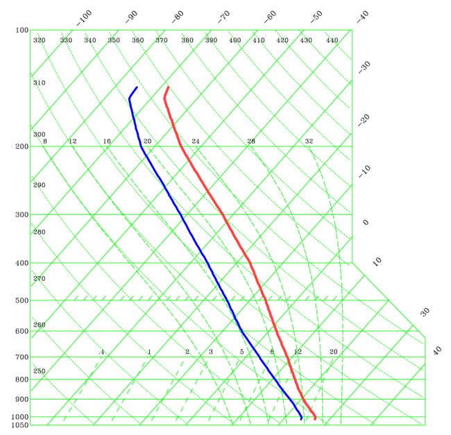
Figure 5.1 shows a skew-T log-p diagram with a mean tropical sounding for the Atlantic hurricane season plotted. The skew-T log-p diagram can be used to investigate changes of state of an air parcel as its pressure changes.
The amount of energy that a particular parcel could achieve by rising from a particular level zi to its LNB is called the convective available potential energy (CAPE) and may be written as

where b is the generalized buoyancy force per unit mass that acts on on the parcel and dl is a unit vector along the path of the displacement. If the parcel rises vertically, this integral may be written

where z measures height (normal to geopotential surfaces) and b is the vertical component of the buoyancy force. Using the equation of state in the form p = ρRTρ where Tρ is the density temperature, and assuming that the environment is in hydrostatic equilibrium, we can show that (see Exercise 5.X)

It follows that CAPEi is proportional to the area enclosed by the density temperature of the lifted parcel and that of the environment, respectively, on a thermodynamic diagram whose coordinates are linear in temperature and in log p. CAPE depends on the initial parcel, i, and on the thermodynamic process assumed in lifting the parcel. It is defined only for those parcels that are positively buoyant somewhere on the sounding.
The amount of work that must be expended to lift a parcel to its level of free convection is called the convective inhibition (CIN) and is given by the integral

Again, if the parcel is lifted vertically, this integral may be written

The negative area represents, in essence, a potential barrier, or potential well, to convection, that prevents it from occurring spontaneously. There is no analogy to this potential barrier in dry convection; this is one distinguishing feature between moist and dry convection, although not only one. The existence of a potential barrier allows CAPE to accumulate under certain meteorological conditions, creating the possibility that it may be released explosively at a later time.
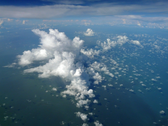
Figure 5.2 shows some photographs of tropical convection in a variety of forms. It is sometimes useful to divided convection into three types, shallow convection, intermediate convection and deep convection as follows.
Shallow convection refers to convective clouds that have a limited vertical extent, with tops perhaps no more than one or two kilometres. Generally such clouds do not precipitate. They are often referred to as "trade-wind cumuli". Theoretical treatments of shallow convection assume that the clouds do not produce precipitation. Fields of shallow convection are important for the larger scale because the convection facilitates mixing, leading to a vertical transport of heat and moisture into the cloud layer and the transport of dry air through intra-cloud subsidence into the subcloud layer. In this way, shallow convection counteracts the drying and warming effects of large-scale subsidence regions. Examples of shallow convection can be seen in all the panels Fig. 5.2 suggesting that such convection is ubiquitous in the tropics.
 (b)
(b)
(c)
 (d)
(d)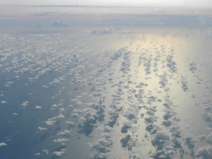
(e)
 (f)
(f)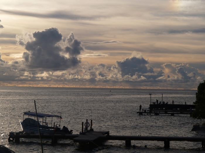
(g)
 (h)
(h)
Intermediate convection refers to convective clouds that produce heavy showers, but which do not extend far enough in the vertical to contain ice. In the tropics the freezing level is around 5.5 km. In these clouds the processes leading to the rain do not involve ice processes. Thus rain drops are produced only by the collision and coalescence of smaller drops. We refer to the rain produced in such clouds as \textit{warm-rain}. Examples include so called cumulus congestus clouds, examples of which are shown in Fig. 5.2 (a), (c) and (e).
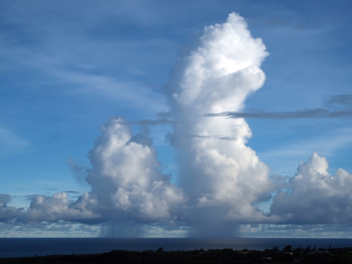
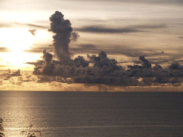
Deep convection refers to precipitating clouds that extend vertically through a significant depth of the troposphere, typically well above the freezing level. Besides producing heavy local precipitation, they may give rise to thunder and lightning. An important characteristic of precipitating convection is the production of strong downdraughts when precipitation evaporates in subsaturated air, or when it melts at the freezing level. An example is shown in the distance in Fig. 5.3(c). Deep convective clouds usually produce extensive anvils of ice particles that often outlive the convective cells that generate them. These anvil clouds take on a dynamics of themselves with slow ascent above the freezing level and subsidence below generated by moderate to weak precipitation below them. There may be significant convergence near the freezing level induced by the sharp increase in the fall speed of hydrometeors as snow melts to form raindrops.
The downdraughts that accompany deep convective systems can have an important stabilizing effect on the subcloud air, making it cooler and drier. However, once a convective cell has developed, lifting of air ahead along the boundaries of the low-level cold outflow can trigger new convection. In this manner, convective systems have a propensity to generate new cells that subsequently aggregate. Over the ocean, surface fluxes of heat and moisture lead to a warming and moistening of the downdraught air on time scales on the order of half a day, thereby restoring convective instability.
The warming of the atmosphere in regions of convection is a result not only of the direct release of latent heat in clouds, but also by the subsidence in the environment of clouds brought about by horizontally-propagating gravity waves. In this way, a whole region including clouds and their environments can undergo warming.
Typical updraughts speeds in deep convection over the oceanic are typically only a few m s-1, somewhat weaker than typical speeds in deep convection over land in the middle latitudes, where updraughtsmay reach 15 m s-1, or more (see Lucas et al. 1994 ). However, tropical clouds are generally deeper than their middle latitude counterparts as the tropopause is several kilometres higher in the tropics. An interesting paper on this topic is that by Zipser (2003) .
An important consideration in understanding the interaction between deep convection and the broadscale flow in tropical disturbances is to realize that deep convection occurs as a result of convective instability. First, some air parcels must be brought to their LFC, either as a result of boundary layer turbulence or as a result of mechanical lifting at the spreading outflow boundary produced by previous convection. Above the LFC, air parcels can rise through the depth of the troposphere in favourable conditions and they may even overshoot their LNB into the lower stratosphere. It turns out that usually, only air parcels below a few 100 m to 1 km have any CAPE so that only these can rise through a deep layer. Thus deep convection typically peels of a layer of warm moist air near the surface and expels (or detrains) it into the upper troposphere near the level of neutral buoyancy. At air parcels rise they entrain air from their environment. The entrained air is generally unsaturated and slightly cooler than the air parcel so that entrainment tends to reduce the amount of buoyancy in the updraught below that which would be predicted by an aerological diagram and tends to lower the LNB.
When an air parcel ascends in a stably stratified environment, it expands and cools. As long as it remains unsaturated it cools at the dry adiabatic lapse rate (10oC km-1) and if a parcel could be lifted dry adiabatically from the surface in the tropics (say with a temperature of 29oC) to the tropopause (say at a height of 15 km), it would have a temperature when it reached the tropopause of -121oC (see Figure 5.3). Since temperatures near the tropical tropopause are typically around -73oC, the air parcel would have a huge negative buoyancy when it got there and the lifting would require a huge amount of work to be done to lift the parcel. Since there is no conceivable mechanism in the atmosphere that could supply the needed work, we must conclude that the air parcel must rise in cloud, where the cooling can be offset by latent heat release, first as condensation occurs and later as freezing occurs.
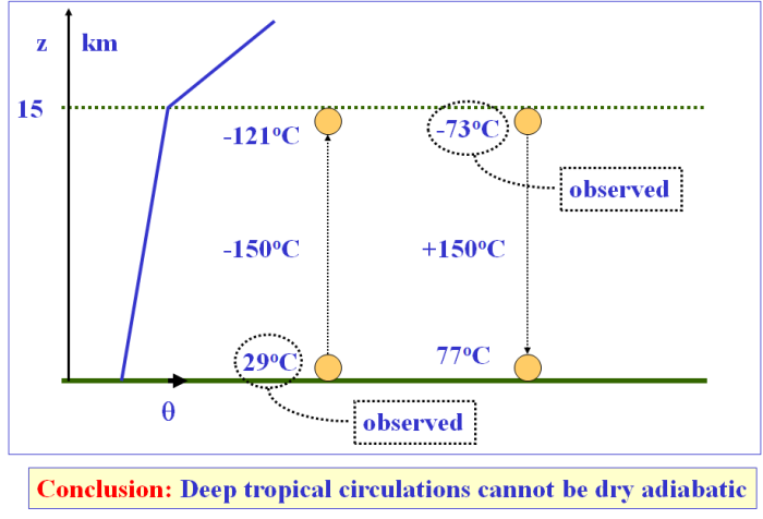
A similar argument can be used to argue that an air parcel cannot descend from the tropopause level to the surface unless it cools to offset the 150oC temperature rise that would be produced as a result of adiabatic compression. Typically, the subsiding air parcel with an initial temperature at the tropopause of -73oC would have to cool radiatively, the normal rate being on the order of 2oC per day. Thus, in order to arrive at the surface with a temperature of 29oC, the parcel would have to cool by 48oC, which could be accomplished only after 24 days. Since an air parcel can rise from the surface to the tropical tropopause in about 20 minutes, mass conservation would require that the area of descent be much larger than the area of ascent.
We have seen that friction effects near the surface in a vortex induce convergence in a shallow boundary layer, with upflow at the top of the boundary layer. While the lifting so produced may bring air parcels to their level of free convection, the ability of the convection rising as a result of the buoyancy that can be achieved to remove the air that is converging will not match, in general, the mass that converges in the boundary layer as a result of friction. If the buoyancy of the convection is too weak, it will be unable to "ventilate" the mass that is converging in the boundary layer and the air that cannot be ventilated will flow radially outwards in a shallow layer above the boundary layer (shallow because the air is typically stably stratified). On the other hand, if the vortex is relatively weak and the buoyancy of deep convection relatively strong, the convection will dominate the inflow in its vicinity and induce local subsidence at radii where the boundary layer inflow cannot supply the air that is being removed by convection. Clearly, a steady state could be envisioned only when the boundary layer is supplying mass at exactly the rate that deep convection can ventilate it. We will return to the issue of a possible steady state later.
Latest version: Munich 13 August 2013