To understand spin-up of a tropical cyclone it is instructive to consider first the way in which a vortex spins down problem as a result of friction. We examine first the essential dynamics of the spin-down problem and proceed then to a scale analysis of the equations with the friction terms included.
The classic vortex spin down problem considers the evolution of an axisymmetric vortex above a rigid boundary normal to the axis of rotation. We will show that the spin down is intimately connected to the Coriolis torques associated with the secondary circulation induced by friction. The direct effect of the frictional diffusion of momentum to the surface is of secondary importance to the spin down in the parameter regimes relevant to tropical cyclones.
In a shallow layer of air near the surface, typically 500 - 1000 m deep, frictional stresses reduce the tangential wind speed and thereby the centrifugal and Coriolis forces, while it can be shown that the force associated with the radial increase of pressure remains largely unchanged. We call this layer the friction layer. The result of the force imbalance is a net inward force that drives air parcels inwards in this layer.
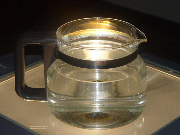
One can demonstrate the foregoing effect by placing tea leaves in a beaker of water and vigorously stirring the water to set it in rotation. After a short time the tea leaves congregate near the bottom of the beaker near the axis as shown in Fig. 4.1: they are swept there by the inflow in the friction layer. Slowly the rotation in the beaker declines because the inflow towards the rotation axis in the friction layer is accompanied by radially-outward motion above this layer. The depth of the friction layer depends on the viscosity of the water and the rotation rate and is typically only on the order of a millimetre or two in this experiment. Because the water is rotating about the vertical axis, it possess angular momentum about this axis. Here angular momentum is defined as the product of the tangential flow speed and the radius. As water particles move outwards above the friction layer, they conserve their angular momentum and as they move to larger radii, they spin more slowly. The same process would lead to the decay of a tropical cyclone if the frictionally-induced outflow were to occur just above the friction layer, as in the beaker experiment. What then prevents the hurricane from spinning down, or, for that matter, what enables it to spin up in the first place? Clearly, if it is to intensify, there must be a mechanism capable of drawing air inwards above the friction layer, and of course, this air must be rotating about the vertical axis and possess angular momentum so that as it converges towards the axis it spins faster. The only conceivable mechanism for producing inflow above the friction layer is the upward ``buoyancy force" in the clouds, the origins of which we examine below.
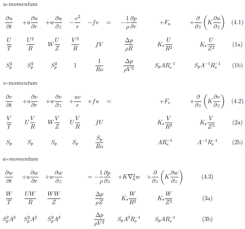
We repeat now the scale analysis of the dynamical equations (3.1)-(3.3) with friction terms added to the right-hand-sides. We have assumed a particularly simple form for friction with K an eddy diffusivity, assumed to be at most a function of z and having typical scale K*. We assume that the air is homogeneous and that the motion is axisymmetric and define velocity scales (U,V,W), length scales (R,Z), and an advective time scale T = R/U as before. Now we assume that p is perturbation pressure and take Δp to be a scale for changes in this quantity. The continuity equation (3.4) yields the same relation between W/Z \sim U/R as before. Then the terms in Eqs. (3.1) to (3.3) have nondimensional scales as shown in Table 4.1.
As in section 3.6 we divide terms in line (2a) by V2/R to obtain those in line (2b) and divide terms in line (3a) by UV/R to obtain those in line (3b). The terms in line (4a) are divided by g to obtain those in line (4b). The terms in lines (b) are then nondimensional. We define a Reynolds number, Re = VZ/K*, which is a nondimensional parameter that characterizes the importance of the inertial to frictional terms, and an aspect ratio A = Z/R, that measures the ratio of the boundary-layer depth to the radial scale. For typesetting reasons we represent the horizontal friction terms (K(∇h2u - u/r2), K(∇h2v - v/r2)) by (Fu, Fv), where ∇h2 = ∂/∂r(r∂/∂r).
Typically, the boundary layer is thin, not more than 500 m to 1 km in depth and the aspect ratio is small compared with unity. Moreover, typical values of K* are on the order of 50 m s-2. Therefore taking V = 50 m s-2, R = 50 km, and Z = 500 m, Re = 5 × 10² and A = 10-2. It follows from line (3b) in Table 4.1 that Δp/(ρV-2) approx max(Sp2A2, SpARe-1) = 4 × 10⁻⁴, assuming that Sp ≈ 1 in the boundary layer. Thus the vertical variation of p across the boundary layer is only a tiny fraction of the radial variation of p above the boundary layer. In other words, to a close approximation, the radial pressure gradient within the boundary layer is the same as that above the boundary layer.
From lines (1a) and (2a) in Table 4.1, we see that a vertical scale Z which makes friction important compared with the other large terms is (K*/f)½ if Ro << 1 and (K*/(V/R))½ if Ro ≈ 1 or larger. The former result gives us the appropriate scaling for the Ekman layer (see Exercise 4.1).
The scale analysis of the w-momentum equation shows that the horizontal pressure gradient in the boundary layer is essentially the same as that above it. Thus we may express the radial pressure gradient in Eq. (4.1) by that of gradient wind above the boundary layer. We assume that the radial flow above the boundary layer is zero or small compared to the gradient wind. Then the u- and v-momentum equations in the boundary layer become:
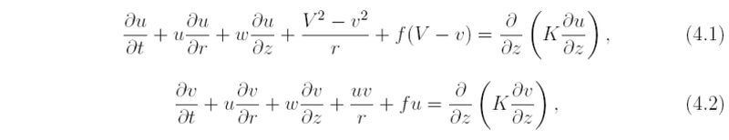
where V(r) is the gradient wind speed above the boundary layer. The vertical velocity in the boundary layer is determined by the continuity equation. Because the boundary layer is typically thin so that density variations across it may be neglected the continuity equation takes the form:

To summarize, the principal simplifications of boundary layer approximations are that the horizontal pressure gradient of the flow above the boundary layer is transmitted unchanged through the boundary layer to the surface and the friction terms are dominated by the vertical derivative term. In the case of a steady boundary layer, the latter assumption changes the character of the flow equations from elliptic to parobolic, which has consequences for the direction of information flow (see later).
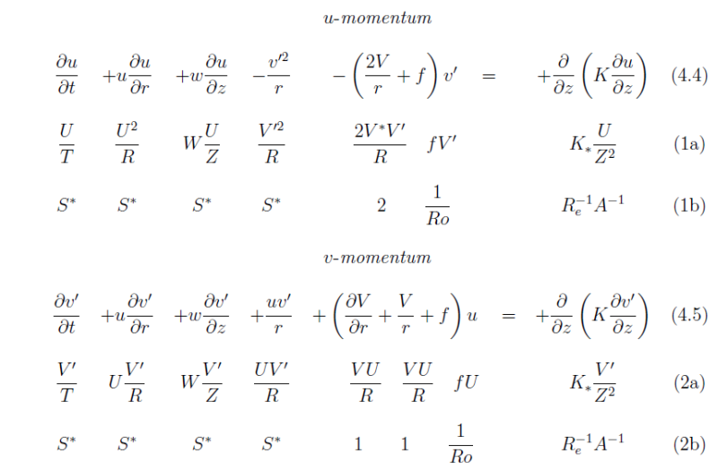
Equations (4.1) and (4.2) may be further simplified by the substitution v = V(r) + v', to become:

We carry out now a scaling of the terms in these equations as shown in Table 4.2. Let U, V* and V' be scales for u, V and v', respectively. We assume that U = V' and define S* = U/V*.
With the background gradient wind balance removed, there is less of a scale separation between the remaining terms in the boundary-layer equations, but further simplifications are possible for certain parameter values if the flow is steady. If S* << 1 and Ro << 1, the equations reduce to the classical Ekman equations, which are explored here in the context of Exercise 4.1. A similar, but more general set of equations is explored in the next section.
If S* << 1 but Ro is of order unity or larger, Eqs. (4.4) and (4.5) may be linearized to give
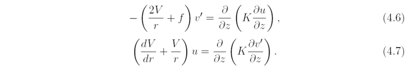
It is interesting to examine this linear approximation even though it turns out that S* may be as large as 0.3 in a tropical cyclone. Thus the neglect of terms of magnitude 0.2-0.3 compared with unity is unlikely to be very accurate. The difference in the coefficients of v' and u on the left-hand-side of Eqs. (4.6) and (4.7) precludes the method normally used to solve the Ekman equations, in which both coefficients reduce to f (Exercise 4.1). However, if we assume that K is a constant, one of the equations may be differentiated twice with respect to z and the remaining equation can be used to eliminate either u or v'. Then each of these quantities satisfies the equation

The solutions have the form x = a exp{αz} where α4 = (I2/K2)exp(iπ + 2nπi), (n = 0, 1, 2, 3 ... ), and a is a constant. Thus the four roots are α = ±(1 ± i)/δ, where δ = (2K/I)½ is the boundary-layer scale thickness. The solutions for v' and u which decay as z → ∞ can be written succinctly in matrix form
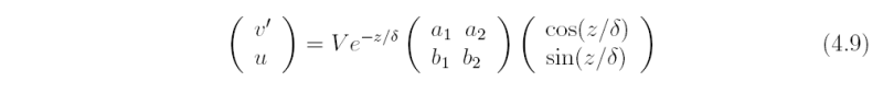
where a1, a2, b2, b2 are constants.
For a turbulent boundary layer like that in a tropical cyclone, an appropriate boundary condition at the surface is to prescribe the surface stress, τ0, as a function of the near-surface wind speed, normally taken to be the wind speed at a height of 10 m, and a drag coefficient, CD. The condition takes the form:

and we shall apply it at z=0 instead of 10 m.
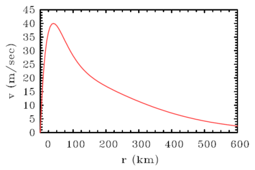
Two relations between these constants may be determined by applying the boundary condition (4.10), remembering that this applies to the total surface wind field (V + v',u). Two further relationships may be obtained by substituting for v' and u in Eq. (4.7). The details form the basis of Exercise (4.4). Given a radial profile of V(r) such as that shown in Fig. 4.2, it is possible to calculate the full boundary-layer solution (u(r,z), v(r,z), w(r,z)) on the basis of Eq. (4.9). The vertical velocity, w(r,z) is obtained by integrating the continuity equation (see Exercise 4.5).
Substituting (4.9) into (4.5) and tidying up the equation gives

where ν = CDRe and Re = Vδ/K is a Reynolds number to the boundary layer. After a little algebra, setting 1 - A = Bexp(iβ} gives an algebraic equation for B and an expression for β in terms of B (see Exercise 4.2). The equation for B may be solved using a Newton-Rapheson algorithm.
The vertical profiles of u(z) and v(z) at a radius of 150 km are shown in Fig. 4.3a and the hodograph thereof is shown in Fig. 4.3b. At this radius Vg is approximately 20 m s-1. Other parameters used for the calculation are f = 5 × 10⁻⁵ s-1, K = 10 m2 s-2 and CD = 0.002. For these values, the boundary layer depth scale, δ = 472 m and the surface values of v and u are about 0.6Vg and 0.3Vg, respectively. Note that, consistent with Eq. (4.6), supergradient winds occur at levels where the curvature of the radial wind (i.e. ∂2z / ∂z2) is positive. At these heights, there is a convergence of stress associated with the vertical turbulent diffusion of radial momentum. In steady conditions, this stress convergence is balanced by the net agradient force.

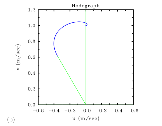
Figure 4.4 shows the isotachs of u and v below a height of 2 km and the vertical velocity at the top of the boundary layer for the tangential wind profile shown in Fig. 4.2. It shows also the radial variation of the boundary layer depth scale, δ. Note that δ decreases markedly with decreasing radius, while the inflow increases. The decrease of δ is simply related to the radial increase in the inertial stability parameter with decreasing radius, but it ignores the likely increase in eddy diffusivity as the wind speed (and hence vertical wind shear) increase. The maximum inflow occurs in this case at a radius of 90 km, 50 km outside the radius of maximum wind speed above the boundary layer, rm. In contrast, the maximum vertical velocity at "large heights" peaks just outside rm. There is a region of weak outflow above the inflow layer, partially overlapping with the region where tangential flow becomes supergradient (i.e. larger than the gradient wind speed).

The scale analysis of the u- and v-momentum equations in Table 4.1 shows that for small Rossby number (Ro << 1), there is an approximate balance between the net Coriolis force and the diffusion of momentum. If K is assumed to be a constant, this balance is expressed by the equations:

and

where (0, V
with the substitution VE = v + iu, where i = √(-1), Eqs. (4.12) and (4.13) reduce to the single differential equation

where VEg is the gradient wind above the boundary layer.
equation (4.14) has the particular integral V = VEg and two complementary functions proportional to exp(±(1 - i)z/δ), where δ = √(2K/f).
the solution of (4.14) that remains bounded as z → ∞ has the form

where A is a complex constant determined by a suitable boundary condition at z = 0.
For a laminar viscous flow, the no-slip boundary condition at z =0 gives A = 1. This is the classical Ekman solution.
Two interesting features of the Ekman solution are the fact that the boundary-layer thickness, measured by δ is a constant and there are regions in the boundary layer where the flow is supergeostrophic, i.e. v > Vg. These are unusual features of boundary layers which are typically regions where the flow is less than that at the top of the layer and which grow in thickness downstream as more and more fluid is retarded. In the Ekman layer, the fluid that is retarded in the downstream direction, but is re-energized in the cross-stream direction by the net pressure gradient force in that direction. The latter occurs because friction reduces the Coriolis force in the boundary layer whereas the radial pressure gradient remains effectively unchanged. The height range where the flow is supergeostrophic is one in which the net radial flow is outwards. As in case of the the linear solution discussed above, the fact that the flow is supergeostrophic is a result of the upward turbulent diffusion of u-momentum, which is largest at low levels, and the convergence of the associated momentum flux. (explanation needs tweaking)
Show that the substitution A = 1-Beiβ in Eq (4.6) leads to the equation

and the β is given by tan β = - νB/(νB + 1)
[Hint: after substitution, equate real and imaginary parts to obtain a pair of simultaneous equations for cosβ and sin β.]
Show that the substitution (4.9) into the boundary condition (4.5) gives the two relationships

and that the substitution into Eq. (4.12) gives two more relationships

where ζa = ζ + f. Show the points (a1, a2) lie on a circle centred at the point (-½,-½) with radius 1/√2 and may be expressed as a1 = cos θ/√2 - ½, a1 = sin θ/√2 - ½. Hence derive an equation for θ.
The frictional boundary layer is a very important feature of a tropical cyclone as it provides a powerful coupling between the primary circulation and the secondary circulation. Moisture enters a hurricane from the sea surface and its radial distribution is strongly influenced by that of the boundary layer winds. Indeed, the boundary layer dynamics and thermodynamics determine the vertical transport of moisture and angular momentum out of the boundary layer and the radial distribution of these quantities on leaving the layer exerts a strong constraint on the radial distribution of buoyancy.
The theory presented in the sections above shows that, at least by itself, the boundary layer leads to vortex spin-down. More precisely, if deep convection in the inner core region of tropical cyclone is collectively too weak to remove all the mass that is converging in the boundary layer, there will be outflow just above the boundary layer and the tangential circulation at the top of the boundary layer will decay. On the other hand, if the convection is sufficiently vigorous, one can envisage a situation in which the convergence of low level air it produces exceeds the rate that can be supplied by the vortex scale boundary level. For reasons to be explained in section 4.6.1, in such conditions, boundary layer theory will not be locally applicable. Of course, the convergence induced by the convection will not be confined just to the boundary layer: it will typically extend through much of the lower half of the troposphere.
While providing a qualitatively correct picture of the frictionally-induced convergence in the boundary layer, the scale analysis above would suggest that the linear approximation is a poor approximation quantitatively in a tropical cyclone strength vortex and that the neglect of the nonlinear terms cannot be justified. Support for this suggestion can be obtained simply, in principle, by calculating the nonlinear terms from the linear solution and comparing them with the magnitude of the linear terms retained. Unfortunately there are a number of issues in formulating the steady boundary layer problem with the nonlinear terms included as discussed in section 4.6.1. Some insight into these issues is provided by examining a slab model for the boundary layer in which a representation of nonlinear terms is possible. Such a model is discussed in section 4.5.
In this section we describe a relatively simple nonlinear model for the tropical cyclone boundary layer of a stationary vortex. The structure of the model is shown schematically in Fig. 4.5. The flow is assumed to be steady and axisymmetric on an f-plane. The boundary layer is assumed to be homogeneous and to have uniform depth h. The flow at the top of the layer is assumed to be in gradient wind balance with tangential wind speed V(r) and zero radial wind speed. The vertically-averaged radial and tangential wind speed components in the boundary layer are denoted by ub and vb. It is straightforward to include a formulation of thermodynamics into the slab model, but we will focus here on the dynamical aspects. As in section 4.3 we use a bulk formula to represent the effects of surface drag.
With the foregoing assumptions we integrate the boundary layer equations with respect to depth and obtain a set of coupled ordinary differential equations governing the radial variation of ub and vb, together with an algebraic equation for wh. These equations may be integrated inwards from some large radius, R, at which V(R) is sufficiently small that the boundary layer can be approximated by the slab form of the Ekman layer, i.e. at this radius the nonlinear acceleration terms, including the centripetal acceleration, may be neglected. With these assumptions we can solve for ub and vb at this radius. The details are given in the next subsections.
For the model configuration described above, the boundary layer equations may be written in flux form as:
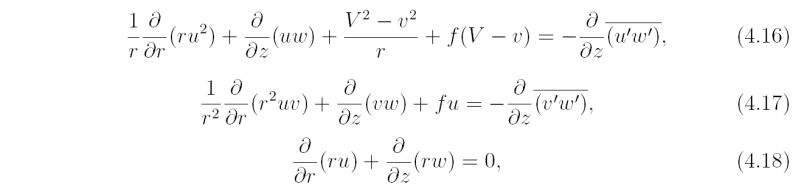
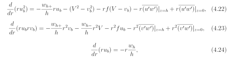
where (u,v,w) is the mean velocity vector in a stationary cylindrical coordinate system (r,λ,z) and prime quantities denote turbulent fluctuations about this mean. Taking the integral of Eqs. (4.20) - (4.22) with respect to z from z = 0 to the top of the boundary layer, z = h, and assuming that h is a constant, we obtain:

Now [ruw]z = h = ru_bwh+ + rUwh-, where U is the radial component of flow above the boundary layer, taken here to be zero, wh+ = (1 / 2)(w_h + |w_h |), and w_{h-} = {1 \over 2}(w_h - |w_h|). Note that wh+ is equal to wh if the latter is positive and zero otherwise, while wh- is equal to wh if the latter is negative and zero otherwise. Carrying out the integrals in Eqs. (4.23)-(4.25) and dividing by h gives
and

which may be written

where a subscript 'b' denotes a mean value through the depth of the boundary layer. Before we can proceed further, we must find a way to represent the turbulent flux terms on the right-hand-side of Eqs. (4.26) - (4.27). We examine this problem in the next section.
The surface momentum flux terms in (4.26) - (4.27) are represented by an empirical bulk drag law:

where CD is a drag coefficient and ub = (ub,vb). This term represents the rate of which momentum is lost to the surface and characterizes the frictional drag imposed by the surface on the air above. Based on the latest available data we use the formula CD = CD0 + CCD1|ub|, where CD0 = 0.7 × 10⁻³ and CD1 = 6.5 × 10⁻⁵ for wind speeds less than 20 m s-1 and CD = 2.0 × 10⁻³. For simplicity we ignore the turbulent momentum fluxes at the top of the boundary layer. Strictly, Eq. (4.26) should be applied at a height of 10 m.
For any dependent variable η
where η is either ub or vb. Then, dividing each by ub, Eqs. (4.26) and (4.27) become

Equations (4.25) and (4.27) - (4.28) form a system of coupled ordinary differential equations that may be integrated radially inward from r = R to find ub and vb as functions of r, given values of these quantities at r = R. The quantity whis obtained by making sure that dub/dr predicted by the radial momentum equation, Eq. (4.27), is consistent with that predicted by the continuity equation, Eq. (4.25)
In the foregoing derivation, Eq. (4.27) is written in the form ubwh-/h} = ubdub/dr + ... and dub/dr is eliminated from this expression using (4.25).
Note that if wh- < 0, wh- = wh-, in which case α = 1. If wh > 0, wh- = 0, in which case α = 0.
Then

where α is zero if the expression in square brackets is negative and unity if it is positive.
We assume that at r = R, far from the axis of rotation, the flow above the boundary layer is steady and in geostrophic balance with tangential wind speed V(R). In addition we take CD to be equal to CD0 + CD1V(R). Then ub and vb satisfy the equations:

A first approximation to the solution may be obtained analytically after setting the first terms on the right-hand-side of each equation to zero, i.e. by neglecting momentum
transport from above. Then the vertical velocity at r = R, wh-(R), can be diagnosed in terms of V and its radial derivative using the continuity equation (4.25). Specifically

When wh-(R) has been determined, Eqs. (4.30) and (4.31) are solved again to find new values of ub and vb and the whole procedure is repeated until stable values are obtained for the four quantities.
With the starting values for ub and vb determined by Eqs. (4.30) and (4.31), Eqs. (4.27)-(4.28) may be solved numerically, given the radial profile V(r).
Figure 4.6 shows an example of a solution for the slab boundary layer using the same radial profile of gradient wind shown in Fig. 4.2. The boundary layer depth is taken to be 1000 m and the starting radius for the calculation, R = 500 km, beyond the radius plotted. Figure 4.6a shows radial profiles of wind components in the boundary layer and at the top of it and Fig. 4.6b shows the vertical velocity at the top of the layer. The general characteristics of the solution are that, beyond a radius of about 60 km, the tangential wind speed, vb, is a few metres per second less than that at the top of the boundary layer, V, while the radial wind speed is inwards and appreciably less than V. The total wind speed |vb| = √(ub2 + vb2) is slightly less than V beyond a radius of about 90 km. At large radii, the mean vertical motion at the top of the boundary layer, wh, is downwards, but subsidence velocities are relatively weak. The subsidence increases with decreasing radius and then decreases again shortly before changing to ascent. The change from subsidence to ascent occurs at a radius of 160 km.
At first, as r decreases, both ub and vb increase in magnitude, as does V. The radial wind speed ub attains a maximum of about 16 m s-1 at a radius of 60 km and then declines rapidly. The decline coincides with the radius at which the tangential wind speed first exceeds V, i.e. where vb becomes supergradient. The solution becomes singular (i.e.ub → 0) at a radius of just over 40 km. The maximum values of vb and wh occur at the radius where the solution breaks down. Less than 2 km before this radius, vb = 47 m s-1 and appears to have peaked, while wh = 3 m s-1, is increasing rapidly, probably tending to become infinite at the radius of breakdown.

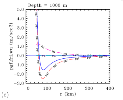
The behaviour of the boundary layer in the slab model depends in a delicate way on the relative importance of various force terms in the radial and tangential momentum equations. The radial profiles of forces in the radial momentum equation (ub × Eq. (4.30)) for the foregoing calculation are shown in Fig. 4.6c. The first term in this equation represents the effects of the downward transport of radial momentum (zero in the present model), and the last represents the frictional stress. Both of these act to reduce the radial inflow. The only terms that can cause a radially-inward acceleration represent the net pressure gradient force per unit mass, (V2 - vb2)/r + f(V - vb) (denoted by pgf in Fig. 4.6), when V > vb. If the flow is supergradient (vb > V), the net pressure gradient acts radially outwards with the other two terms, which accounts for the rapid decline in ub just before the solution breaks down. Beyond a radius of about 80 km the pgf increases with decreasing r, the increase being more rapid than the frictional force (denoted by fri). The increase in vb is assisted by the downward transfer of tangential momentum from above, ub × the term wh-(vb - V)/h in Eq. (4.31), which is denoted by wu in Fig. 4.6c. However, this term makes only a small contribution to the radial force balance in the boundary layer.
The development of wind speeds in the boundary layer larger than those above may seem surprising at first sight, but is consistent with the observation that in tropical cyclones, the maximum tangential wind occurs at low levels, near the top of the strong inflow layer. In the absence of frictional stresses, converging rings of air would conserve their absolute angular momentum and spin faster (section 3.5). Typically, in the boundary layer, they still spin faster, but the rate at which vb increases is reduced by the frictional torque, represented by the last term in Eq. (4.31). From a Lagrangian perspective, the development of supergradient winds requires a sufficiently large radial displacement of air parcels in the boundary layer, which in turn, requires sufficiently large, radially-inward wind speeds. The slower air parcels spiral inwards, the longer tracks they have along which friction can act to reduce vb. This effect is contained in the terms proportional to the inverse of ub in Eq. (4.31).
For the typical tangential wind profile used for the calculation, vb increases faster than V as r decreases inside a radius of about 200 km. In this region, pgf decreases faster than wu + fri so that eventually the net radial force pgf - wu - fri changes sign. This change occurs well before the radius of maximum V is reached. When pgf - wu - fri becomes positive, the radial inflow decelerates, but vb continues to increase as columns of air continue to move inwards. Eventually, pgf tends to zero and the net outward force, primarily due to friction, becomes relatively large so that the inflow decelerates rapidly and vertical velocity at the top of the boundary layer increases dramatically.
In general, the net inward pressure gradient force increases with the degree to which the tangential flow in the boundary layer is subgradient (i.e. with the magnitude of V - vb), which in turn increases as the effective frictional torque increases to reduce vb. This torque is inversely proportional to the boundary-layer depth, since the surface stress is then spread over a shallower layer. It follows that shallower boundary layers favour lower tangential wind speeds, but larger radial wind speeds, because, at least in the outer part of the vortex, they lead to a larger net inward pressure gradient compared with the radial component of friction. At inner radii the situation is different. There, large radial wind speeds favour large tangential wind speeds because then air parcels may penetrate rapidly to small radii, with minimal reduction of vb by the frictional torque as discussed above.
Decreasing the vortex intensity has a similar effect to increasing the boundary layer depth. Calculations for different values of the maximum tangential wind speed at the top of the boundary-layer, Vm, show that as Vm decreases, so does the strength of the maximum supergradient wind speeds. Further, below some threshold in Vm, the solution does not become singular and the equations may be integrated arbitrarily close to the rotation axis. For the parameters chosen for the solution discussed above, the threshold value of Vm is a little below 24 m s-1. The solution for Vm = 23 m s-1 is shown in Fig. 4.6d. In this case, vb remains close to V, oscillating about it, and ub is a much smaller fraction of V at each radius than for Vm = 40 m s-1 (cf Fig. 4.6a). At the same time, wh remains finite, attaining a maximum value of 1.4 m s-1 at a radius of 47 km (not shown).
In this webpage we have examined two models for the boundary layer, a steady linear model which represents the vertical structure of the flow and a steady slab model that includes nonlinear terms, but represents only the vertically averaged properties of the boundary layer. Neither models are accurate in the sense that one would be comfortable to use them as part of a forecast model, but they provide a useful framework for understanding important aspects of the boundary layer behaviour.
The linear solution is limited because, as indicated by the scale analysis performed in section 4.2, the nonlinear terms cannot be ignored at high wind speeds. A limitation of the slab model is the vertical averaging, which may introduce errors in estimating the nonlinear terms. Moreover, when applying the surface boundary condition, one should use the wind at a height of 10 m and not the boundary-layer average wind speed. Notwithstanding these limitations, both models illustrate important features of the boundary layer.
The slab model, for example, illustrates the development of supergradient winds at inner radii and how these may lead to a rapid deceleration of the inflow with an accompanying large increase in the vertical velocity at the top of the boundary layer. The model indicates that the development of supergradient winds in the boundary layer is because of rapid inward radial displacements of air parcels with minimal loss of absolute angular momentum. This process occurs in more sophisticated tropical cyclone models (see Chapter 7) and explains why the maximum tangential winds are located at low levels in real storms (Chapter 2). The linear model produces an elevated layer of supergradient winds at all radii. This layer is associated with the vertical diffusion of inward radial momentum and the generalized Coriolis force that accompanies this diffused momentum.
The slab boundary layer model illustrates an important feature of the full steady boundary layer equations, namely their parabolic nature so that information propagates radially inwards where there is inflow and radially outwards where there is outflow. The implications would be that if there is a region of deep convection removing air from low levels at some inner radii, the boundary layer outside this radius, if governed by the boundary layer equations, cannot know about the removal. The implications would be that boundary layer theory is not valid in such regions.
Another attractive feature of the slab model is the relative ease with which thermodynamics quantities and/or time dependence effects can be incorporated.
The occurrence of supergradient winds in the inner core region predicted by the slab boundary layer solution is suggestive that boundary layer theory may have problems in this region as the boundary layer would be funnelling tangential momentum upwards that is not in balance with the pressure gradient above the boundary layer. However, boundary layer theory \textit{assumes} that the winds above the boundary layer are in approximate gradient wind balance. This assumption will not be valid where there is upward motion out of the boundary layer and suggests that it is incorrect to prescribe the horizontal wind components at the top of the boundary layer as is often done (for example, it is done in the linear solution, but is not necessary in the slab model). In essence, the top of the boundary layer must be regarded as an open boundary for the boundary layer, which means that the horizontal wind at this level must be determined by the boundary layer itself and not prescribed. For these reasons it would seem inappropriate to judge the integrity of the slab model based on a comparison with a model whose integrity is, itself, in question! Time-dependent numerical model simulations show that there is an adjustment region where the flow exits the boundary layer and ascends into the eyewall ... (see Chapter 7).
Thermodynamics of the boundary are important also and are easy to incorporate in the slab model.
Derive the linear approximation to the steady slab boundary layer, analogous to Eqs. (4.6) and (4.7).
Show that the upper boundary condition that the vertical gradient of the horizontal velocity components is zero at the top of the boundary layer is equivalent to prescribing the radial wind component to be zero and the tangential component to be the gradient value.
Latest version: Munich 20 July 2014