In geographical terminology "the Tropics" refers to the region of the earth bounded by the Tropic of Cancer (lat. 23.5oN)
and the Tropic of Capricorn (lat. 23.5oS). These are latitudes where the sun reaches the zenith just once at the summer
solstice. An alternative definition would be to choose the region 30oS to 30oN, thereby dividing the earth's
surface into equal halves. Defined in this way the tropics would be the source of all the angular momentum of the atmosphere and
most of the heat. But is this meteorologically sound? Some parts of the globe experience "tropical weather" for a part of the year
only - southern Florida would be a good example. While Tokyo (36oN) frequently experiences tropical cyclones, called
“typhoons” in the northwestern Pacific region, Sydney (34oS) never does.
Riehl (1979) chooses to define the meteorological "tropics" as those parts of the world where atmospheric processes differ
significantly from those in higher latitudes. With this definition, the dividing line between the "tropics" and the
“extratropics” is roughly the dividing line between the easterly and westerly wind regimes. Of course, this line varies
with longitude and it fluctuates with the season. Moreover, in reality, no part of the atmosphere exists in isolation and interactions
between the tropics and extratropics are important.
Figure 1. Principal land and ocean areas between 40oN and 40oS.
The solid line shows the 18oC sea level isotherm for the coolest month; the dot-dash line is where
the mean annual range equals the mean daily range of temperature. The shaded
areas show tropical highlands over 1000 m. (From Nieuwolt, 1977).
Figure 1 shows a map of the principal land and ocean areas within 40o latitude
of the equator. The markedly non-uniform distribution of land and ocean areas in
this region may be expected to have a large influence on the meteorology of the
tropics. Between the Western Pacific Ocean and the Indian Ocean, the tropical land
area is composed of multitude of islands of various sizes. This region, to the north
of Australia, is sometimes referred to as the “Maritime Continent”, a term that was
introduced by Ramage (1968). Sea surface temperatures there are particularly warm
providing an ample moisture supply for deep convection. Indeed, deep convective
clouds are such a dominant feature of the Indonesian Region that the area has been
called “the boiler-box”Ø of the atmosphere. The Indian Ocean and West Pacific region
with the maritime continent delineated is shown in Fig. 2.
Figure 2. Indian Ocean and Western Pacific Region showing the location of the Maritime Continent (the region
surrounded by a dashed closed curve).
1.1 A tour of the tropics in satellite pictures
Figure 3 shows some typical infra red satellite imagery from geostationary satellites located at different longitudes.
The white areas in the tropics and subtropics indicate cold cloud tops and correspond with cirrus cloud in the high troposphere.
Much of which is produced by deep convection in which air is rapidly ascending. The individual convective updraughts cover
a much smaller fractional area of the area covered by the cirrus, which blows away from the convection. Deep convection
is frequently concentrated in clumps referred to as cloud clusters. Sometimes these have the form of organized convective
systems, an exterme case being that of a tropical cyclone. Such a system is seen in the upper left panel, to the northeast
of the island of Madagascar. <\p>
The dark areas in the tropics and subtropics correspond with regions devoid of cloud, or at least high cloud. These are
regions in which air is slowly subsiding.
The grey areas, mainly in the subtropics and at higher latitudes correspond with regions of low cloud, typically stratus
or strato-cumulusor at least high cloud. Such areas are prominent over the colder waters south and west of Australia in the
upper right panel and to the west of the North and South American Continents.
The band of white cloud just north of the equator in the lower panel marks the Intertropical Convergence Zone (often
referred to as the ITCZ). This cloud marks a strip of deep convective systems that constitute the ascending brance of the
Hadley circulation to be discussed later.
Figure 3. Infra red satellite imagery from geostationary satellites located at different longitudes.
Animations of Satellite imagery
Click here
for an animation of the month July 2003 from the European geostationary satellite
centered on the Equator in European longitudes. (470 Mb)
Click here
for an animation of the tropical Atlantic region during the 2004 hurricane season.
(510 Mb)
1.2 Precipitation and energetics
Figure 4 shows the distribution of mean incoming and outgoing radiation at the edge of the atmosphere averaged zonally and
over a year. If the earth-atmosphere system is in thermal equilibrium, these two streams of energy must balance. It is
evident that there is a surplus of radiative energy in the tropics and a net deficit in middle and in high latitudes,
requiring on average a poleward transport of energy by the atmospheric circulation. Despite the surplus of radiative
energy in the tropics, the tropical atmosphere is a region of net radiative cooling (Newell et al., 1974). The fact is
that this surplus energy heats the ocean and land surfaces and evaporates moisture. In turn, some of this heat finds
its way into the atmosphere in the form of sensible and latent heat and it is energy of this type that is transported polewards
by the atmospheric circulation.
Figure 4. Zonally averaged components of the absorbed solar flux and emitted thermal infrared flux at the
top of the atmosphere. + and - denote energy gain and loss, respectively. (From Vonder Haar and Suomi, 1971, with
modifications).
Figure 5 shows the zonally-averaged distribution of mean annual precipitation as function of latitude. Note that the
precipitation is higher in the tropics than in the extratropics with a maximum a few degrees north of the equator.
When precipitation occurs, i.e. a net amount of condensation without re-evaporation, then latent heat is released.
The implication is that latent heat release may be an important effect in the tropics.
Figure 5. Mean annual precipitation as a function of latitude. (After Sellers, 1965).
1.3 The zonal mean circulation (Hadley circulation), Inter-Tropical Convergence Zone (ITCZ)
Various diagrams have been published depicting the mean meridional circulation of the atmosphere (see. e.g. Smith, 1993, Ch. 2).
While these differ in detail, especially in the upper troposphere subtropics, they all show a pronounced Hadley cell with convergence
towards the equator in the low-level trade winds, rising motion at or near the equator in the so-called equatorial trough,
which is co-located with the ITCZ, poleward flow in the upper troposphere and subsidence into the subtropical high pressure zones
(Fig. 6).
Figure 6. The mean meridional circulation and main surface wind regimes. (From Defant, 1958).
The ITCZ is a narrow zone paralleling the equator, but lying at some distance from it, in which air from one hemisphere
converges towards air from the other to produce cloud and precipitation. It is characterized by low pressure and cyclonic relative
vorticity in the lower troposphere. Usually the ITCZ is well marked only at a small range of longitudes at any one time.
Figure 7 shows a case of an ITCZ marked by a very narrow line of deep convection across the Atlantic ocean, a little north of the Equator,
while Fig. 8 shows an unusual case with the ITCZ stretching across much of the Pacific Ocean.
Figure 7. Visible satellite imagery from the EUMETSAT geostationary satellite at 0600 GMT on 19 May 2000 showing a well-formed ITCZ across the Atlantic Ocean.
Figure 8. Visible satellite imagery from the two geostationary satellites at 2100 GMT on 14 May 2003 showing a well-formed ITCZ across the entire Pacific Ocean.
Figure 9 shows the zonally-averaged zonal wind component at 750 mb and 250 mb during June, July and August (JJA) and December, January
and February (DJF). The most important features are the separation of the equatorial easterlies and middle-latitude westerlies and the
variation of the structure between seasons. In particular, the westerly jets are stronger and further equatorward in the winter hemisphere.
The rather irregular distribution of land and sea areas in and adjacent to the tropics gives rise to significant variation of the flow with
longitude so that zonal averages of various quantities may obscure a good deal of the action!
Figure 9. Mean seasonal zonally averaged wind at 250 mb and 750 mb for (a) the
equinox, (b) JJA, and (c) DJF as a function of latitude. The dashed line indicates
the tropospheric vertical average. Units are m s-1. (Adapted from Webster, 1987b).
1.4 Data network in the Tropics
One factor that has hampered the development of tropical meteorology is the relatively
coarse data network, especially the upper air network, compared with the network available in the extra-tropics, at least in the
Northern Hemisphere. This situation is a consequence of the land distribution and hence the regions of human
settlement.
The main operational instruments that provide detailed and reliable information on the vertical structure of the atmosphere are
radiosondes and rawinsondes. Figure 10 shows the distribution and reception rates of radiosonde reports that were received by the
European Centre for Medium Range Weather Forecasts (ECMWF) during April 1984. The northern hemisphere continents are well covered
and reception rates from these stations are generally good. However, coverage within the tropics, with certain notable exceptions,
is minimal and reception rates of many tropical stations is low. Central America, the Caribbean, India and Australia are relatively
well-covered, with radiosonde soundings at least once a day and wind soundings four times a day. However, most of Africa, South America
and virtually all of the oceanic areas are very thinly covered. The situation at the beginning of the 21st century is much the same.
Figure 10. Distribution and reception rate of radiosonde ascents, from land stations,
received at ECMWF during April 1984. Upper panels are for 12 UTC; lower panels for 00 UTC.
Satellites have played an important role in alleviating the lack of conventional
data, but only to a degree. For example, they provide valuable information on
the location of tropical convective systems and storms and can be used to obtain
"cloud-drift" winds. The latter are obtained by calculating the motion of small
cloud elements between successive satellite pictures. A source of inaccuracy lies in
the problem of ascribing a height to the chosen cloud elements. Using infra-red
imagery one can determine at least the cloud top temperature which can be used to
infer the broad height range. Generally use is made of low level clouds, the motion
of which is often ascribed to the 850 mb level (approximately 1.5 km), and high level
cirrus clouds, their motion being ascribed to the 200 mb level (approximately 12
km). Clouds with tops in the middle troposphere are avoided because it is less clear
what their "steering level" is.
Satellites instruments have been developed also to obtain vertical temperature
soundings throughout the atmosphere, an early example being the TOVS instrument
(TIROS-N Operational Vertical Sounder) described by Smith et al. (1979), which is
carried on the polar-orbiting TIROS-N satellite. While these data do not compete
in accuracy with radiosonde soundings, their areal coverage is very good and they
can be valuable in regions where radiosonde soundings are sparse.
A further important source of data in the tropics arises from aircraft wind reports,
mostly from jet aircraft which cruise at or around the 200 mb level. Accordingly,
much of our discussion will be based on the flow characteristics at low and high levels
in the troposphere where the data base is more complete.
1.5 Field experiments
The routine data network in the tropics is rarely adequate to allow an in-depth
study of many of the important weather systems that occur there. For this reason, many
field experiments have been carried out to investigate particular phenomena in detail.
These have varied in size and scope. One early data set was obtained in the
Marshall Islands in 1956, and was used by Yanai et al. (1976) to diagnose the effects
of cumulus convection in the tropics. A further experiment on the same theme, the
Barbados Oceanographical and Meteorological EXperiment (BOMEX), was carried
out in 1969 (Holland and Rasmussen, 1973). Several large field experiments were or
ganized under the auspices of the Global Atmospheric Research Programme (GARP),
sponsored by the World Meteorological Organization - (WMO) and other scientific
bodies (see Fleming et al., 1979). The programme included a global experiment,
code-named FGGE (The First GARP Global Experiment), which was held from December
1978 to December 1979. In turn, this included two special experiments to
study the Asian monsoon and code-named MONEX (MONsoon EXperiments). The first phase,
Winter-MONEX, was held in December 1978 and focussed on the Indonesian
Region (Greenfield and Krishnamurti, 1979). The second phase, Summer-
MONEX, was carried out over the Indian Ocean and adjacent land area from May
to August 1979 (Fein and Kuettner, 1980).
A forerunner of these experiments was GATE, the GARP Atlantic Tropical Experiment,
which was held in July 1974 in a region off the coast of West Africa. Its
aim was to study, inter alia, the structure of convective cloud clusters that make
up the Inter-Tropical Convergence Zone (ITCZ) in that region (see Kuettner et al.,
1974).
More recently, the Australian Monsoon EXperiment (AMEX) and the Equatorial
Mesoscale EXperiment (EMEX) were carried out concurrently in January-February
1987 in the Australian tropics, the former to study the large-scale aspects of the
summertime monsoon in the Australian region, and the latter to study the structure
of mesoscale convective cloud systems that develop within the Australian monsoon
circulation. Details of the experiments are given by Holland et al. (1986) andWebster
and Houze (1991).
Another large experiment was TOGA-COARE. TOGA
stands for the Tropical Ocean and Global Atmosphere project and COARE for the
Coupled Ocean-Atmosphere Response Experiment. The experiment was carried out
between November 1992 and February 1993 in the Western Pacific region, to the east
of New Guinea, in the so-called warm pool region. The principal aim was "to gain
a description of the tropical oceans and the global atmosphere as a time-dependent
system in order to determine the extent to which the system is predictable on time
scales of months to years and to understand the mechanisms and processes underlying
this predictability" (Webster and Lukas, 1992).
1.6 Longitudinal dependence of the circulation in the Tropics: Macroscale circulations
Figure 11 shows the mean wind distribution at 850 mb and 200 mb for JJA. These levels characterize the lower and upper troposphere,
respectively. Similar diagrams for DJF are shown in Fig. 12. At a first glance, the flow patterns show a somewhat complicated structure,
but careful inspection reveals some rather general features.
Figure 11. Mean wind fields at 850 mb and 200 mb during JJA (Based on NCEP Reanalysis data).
At 850 mb there is a cross-equatorial component of flow towards the summer hemisphere, especially in the Asian, Australian and
(east) African sectors. This flow, which reverses between seasons, constitutes the planetary monsoons (see section 1.8 below).
In the same sectors in the upper troposphere the flow is generally opposite to that at low levels, i.e., it is towards the winter
hemisphere, with strong westerly winds (much stronger in the winter hemisphere) flanking the more meridional equatorial flow.
Both the upper and lower tropospheric flow in the Asian, Australian and African regions indicate the important effects of the
land distribution in the tropics. Over the Pacific Ocean, the flow adopts a different character. At low levels it is generally
eastward while at upper levels it is mostly westward. Thus the equatorial Pacific region is dominated by motions confined to a
zonal plane. Note the strong easterly flow along the Equator in the central Pacific in both seasons. These are associated
with the Walker circulation discussed below.
In JJA, the upper winds near the equator are mostly easterly, rather than westerly as suggested by Fig. 6. This feature is
consistent with the fact that mean position of the upward branch of the Hadley circulation lies north of the Equator and, as shown
below, it is dominated by the circulation in the Asian region. In DJF, the upper winds at the Equator are generally westerly in
the eastern hemisphere and westerly in the western hemisphere.
Figure 12. As in Fig. 1.11, but for DJF.
In constructing zonally-averaged charts, an enormous amount of structure is "averaged-out". To expose some of this structure while
still producing a simpler picture than the wind fields, we can separate the three-dimensional velocity field into a rotational part
and a divergent part (see e.g. Holton, 1972, Appendix C). Thus
Here ψ is a streamfunction and χ a velocity potential. The contribution k ∧ ∇ ψ is
rotational with ∇ ∧ (k ∧ ∇ ψ) = k∇2ψ, but nondivergent, whereas,
∇ χ is irrotational, but has divergence ∇2χ. Because of this last property, examination of the velocity
potential is especially useful as a diagnostic tool for isolating the divergent circulation. It is this part of the circulation
that responds directly to the large-scale heating and cooling of the atmosphere.
Figure 13 shows the distribution of the upper-tropospheric mean seasonal velocity potential χ and arrows denoting the divergent
part of the mean seasonal wind field during summer and winter. Two features dominate the picture. These are the large area of negative
χ centred over southeast Asia in JJA and the equally strong negative region over Indonesia in DJF. These negative areas are
located over positive χ centres at low levels (Krishnamurti, 1971, Krishnamurti et al., 1973). Moreover, the two areas dominate all
other features.
Figure 13. Distribution of the upper tropospheric (200 mb) mean seasonal velocity potential (solid lines) and
arrows indicating the divergent part of the mean seasonal wind which is proportional to ∇2χ.
(Adapted from Krishnamurti et al., 1973).
The wind vectors indicate distinct zonal flow in the equatorial belt over the Pacific and Indian Oceans and strong meridional flow
northward into Asia and southward across Australia. The meridional flow is strongest in these sectors (i.e., in regions of strongest
meridionally-orientated ∇ χ) and shows that the Hadley cell is actually dominated by regional flow at preferred longitudes.
When interpreting the χ-fields, a note of caution is appropriate. Remember that ∇ ⋅ V = -∇2χ
and that |w| ∝ |∇ ⋅ V|. Therefore centres of maximum or minimum χ do not coincide with centres of
maximum or minimum vetical velocity, w. The latter occur where ∇2χ is a maximum or minimum.
The seasonal changes in the broadscale upper-level divergence patterns indicated in Fig. 13 are reflected in the seasonal migration
of the diabatic heat sources shown in Fig. 14. These heat sources are identified by regions of high cloudiness, itself characterized by
regions with low values (∼225 W m-2) of outgoing long-wave radiation (OLR) measured by satellites. The assumption is that high
cloudiness (cold cloud tops) arises principally from deep convection heating and can be used as a proxy for this.
Figure 14. Seasonal migration of the diabatic heat sources during the latter half of the year (July-February,
denoted by matching numerals). The extent of the diabatic heat sources is determined from the area with OLR values less than
225 W m-2 from monthly OLR climatology and is approximately proportional to the size and orientation of the schematic
drawings. (Adapted from Lau and Chan 1983)
Krishnamurti's arrows in Fig. 13 are somewhat misleading as they refer only to the wind direction and not its magnitude. It is possible
to study the flow in the equatorial belt by considering a zonal cross-section (longitude versus height) along the equator with the zonal
and vertical components of velocity plotted. The mean circulation in such a cross-section is shown in Fig. 15. Strong ascending motion
occurs in the western Pacific and Indonesian region with subsidence extending over most of the remaining equatorial belt. Exceptions are
the small ascending zones over South America and Africa. It should be noted that the Indonesian ascending region lies to the east of the
velocity potential maximum in Fig. 13, in the area where ∇2χ is largest. The dominant east-west circulation is often
called the Walker Circulation.
Figure 15. Schematic diagram of the longitude-height circulation along the equator.
The surface and 200 mb pressure deviations are shown as dashed lines. Clouds indicate
regions of convection. Note the predominance of the Pacific Ocean - Indonesian
cell which is referred to as the Walker Circulation. (From Webster, 1983)
Also plotted in Fig. 15 are the distributions of the pressure deviation in the upper and lower troposphere. These are
consistent with the sense of the large-scale circulation, the flow being essentially down the pressure gradient.
Figure 15 displays significant vertical structure in the large scale velocity field. Data indicate that the tropospheric wind field
possesses two extrema: one in the upper troposphere and one in the lower troposphere. A theory of tropical motions will have to account
for these large horizontal and vertical scales. Indeed, it is interesting to speculate on the reason for the large scale of the structures
which dominate the tropical atmosphere. Their stationary nature, at least on seasonal time scales, suggests that they are probably forced
motions, the forcing agent being the differential heating of the land and ocean or other forms of heating resulting from it.
There is a considerable amount of observational evidence to support the heating hypothesis. For example, Fig. 16 shows the distribution
of annual rainfall throughout the tropics. It is noteworthy that the heaviest falls occur in the Indonesian and Southeast Asian region
with a distribution which corresponds to the velocity potential field shown earlier. One is led to surmise that the common ascending
branch of the Hadley cell and Walker cell is driven in some way by latent heat release.
Figure 16. Distribution of annual rainfall in the tropics. Contour values marked in
cm/day. (From ... )
It is a separate problem to understand why the maximum latent heat release would be located in the Indonesian region.
Figures 17 and 18 point to a solution.
Figure 17 shows the distribution of mean annual surface air temperature. The pattern possesses considerable longitudinal variation,
but correlates well with the sea surface temperature (SST) distribution shown in Fig. 18. Of great importance is the 8-10oC
longitudinal temperature gradient across the Pacific Ocean. The air mass over the western Pacific should be much more unstable to
convection than that overlying the cooler waters of the eastern Pacific.
Figure 17. Mean annual surface air temperature in the tropics (Units oC. (From ... )
Figure 18. Annual global mean sea surface temperature. (From ... )
It is important to remember that the seasonal or annual mean fields shown above possesses both temporal and spatial variations on
even longer time scales (see section 1.6). Figure 19 shows the mean annual temperature range of the air near sea level. It is
significant that in the equatorial belt, the temperature variations are generally very small, perhaps an order of magnitude smaller
than those observed at higher latitudes. This is true for both land and sea areas. We may conclude that the variations with longitude
shown earlier will be maintained. On the other hand, at higher latitudes, the near surface temperature over the sea possesses a
relatively large amplitude variation which is surpassed only by the temperature variation over land.
Figure missing
Figure 19. Mean annual surface air temperature range in the tropics (Units oC)
Figure 19 shows only the amplitude of the variation and gives no details of its phase. In fact, the ocean temperature at higher latitudes
lags the insolation by some 2 months. Continental temperatures lag by only a few weeks.
1.7 More on the Walker circulation
Figure 20 shows a closer view of the Walker circulation with ascent over the warm pool region and subsidence over the cooler waters
of the eastern Pacific. Over the Pacific the flow is easterly at low levels and westerly at upper levels. The term "Walker Circulation"
appears to have been first used by Bjerknes (1969) to refer to the overturning of the troposphere in the quadrant of the equatorial
plane spanning the Pacific Ocean and it was Bjerknes who hypothesized that the "driving mechanism" for this overturning is condensational
heating over the far western equatorial Pacific where SSTs are anomalously warm. The implication is that the source of precipitation
associated with this driving mechanism is the local evaporation associated with the warm SSTs. This assumption was questioned by
Cornejo-Garrido and Stone (1977) who showed on the basis of a budget study that the latent heat release driving the Walker Circulation
is negatively-correlated with local evaporation, whereupon moisture convergence from other regions must be important.
Figure 20. A close-up view of the Walker circulation showing ascent over the warm
pool region and subsidence over the cooler waters of the eastern Pacific. The flow is
easterly at low levels and westerly at upper levels.
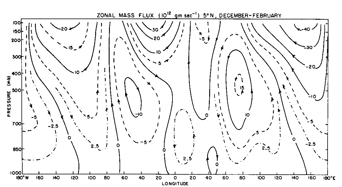
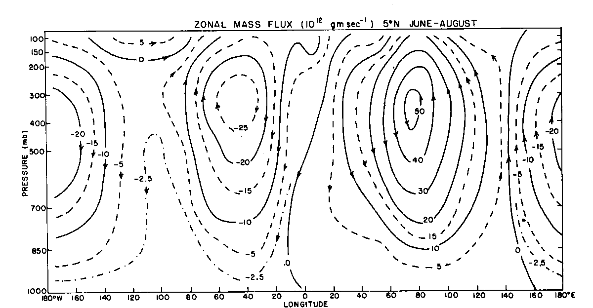
Newell et al. (1974) defined the Walker Circulation as the deviation of the circulation in the equatorial plane from the zonal average.
Figure 21, taken from Newell et al., shows the contours of zonal mass flux averaged over the three month period December 1962 -
February 1963 in a 10.S wide strip centred on the equator. In this representation there are five separate circulation cells visible
around the globe, but the double cell whose upward branch lies over the far western Pacific is the dominant one. A similar diagram
for the northern summer period June to August (Fig. 21b) shows only three cells, but again the major rising branch lies over the
western Pacific. As we shall see, the circulation undergoes significant fluctuations on both interannual (1.8) and intraseasonal (1.9)
time scales.
(a)
(b)
Figure 21. Deviations of the zonal mass flux, averaged over the latitude belt 0oN -
10oN, from the zonal mean. for the periods (a) December - February, and (b) June-August calculated by Newell et al. (1974). Contours do not correspond with
streamlines, but give a fairly good representation of the velocity field associated with
the Walker Circulation.
1.8 El Niño and Southern Oscillation
There is considerable interannual variability in the scale and intensity of the Walker Circulation, which is manifest in the so-called
Southern Oscillation (SO). The latter is associated with fluctuations in sea level pressure in the tropics, monsoon rainfall, and the
wintertime circulation over the Pacific Ocean. It is associated also with fluctuations in circulation patterns over North America and
other parts of the extratropics. Indeed, it is the single most prominent signal in year-to-year climate variability in the atmosphere.
The SO was first described in a series of papers in the 1920s by Sir Gilbert Walker (Walker, 1923, 1924, 1928) and a review and references
are contained in a paper by Julian and Chervin (1978). The latter authors use Walker's own words to summarize the phenomenon. "By the
southern oscillation is implied the tendency of (surface) pressure at stations in the Pacific (San Francisco, Tokyo, Honolulu, Samoa
and South America), and of rainfall in India and Java ... to increase, while pressure in the region of the Indian Ocean (Cairo, N.W.
India, Darwin, Mauritius, S.E. Australia and the Cape) decreases..." and "We can perhaps best sum up the situation by saying that there
is a swaying of pressure on a big scale backwards and forwards between the Pacific and Indian Oceans ... ".
Figure 22a depicts regions of the globe affected by the SO. It shows the simultaneous correlation of surface pressure variations at
all places with the Darwin surface pressure. It is clear, indeed, that the "sloshing" back and forth of pressure which characterizes
the SO does influence a very large area of the globe and that the "centres of action", namely Indonesia and the eastern Pacific, are
large also.
(a)
(b)
Figure 22. The spatial variation of the simultaneous correlation of surface pressure variations at all points with the
Darwin surface pressure (upper panel). Shaded areas show negative correlations. The lower panel shows the variation of the normalized
Tahiti-Darwin pressure difference on the Southern Oscillation Index. (From Webster, 1987b)
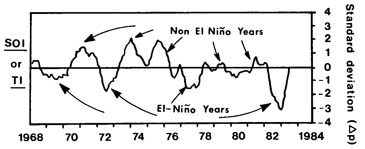
Figure 1.22b shows the variation of the normalized Tahiti-Darwin pressure anomaly difference, frequently used as a Southern Oscillation
Index (SOI), which gives an indication of the temporal variation of the phase of the SO. For example, a positive SOI means that pressures
over Indonesia are relatively low compared with those over the eastern Pacific and vice versa.
It was Bjerknes (1969) who first pointed to an association between the SO and the Walker Circulation, although the seeds for this
association were present in the investigations by Troup (1965). These drew attention to the presence of interannual changes in the
upper troposphere flow over the tropics associated with the SO and indicated that the anomalies in the flow covered a large range of
longitudes. Bjerknes stated:
"The Walker Circulation ... must be part of the mechanism of the still larger 'Southern Oscillation' statistically defined by
Sir Gilbert Walker ... whereas the Walker Circulation maintains east-west exchange of air covering a little over an earth
quadrant of the equatorial belt from South America to the west Pacific, the concept of the Southern Oscillation refers to the
barometrically-recorded exchange of mass along the complete circumference of the globe in tropical latitudes. What distinguishes
the Walker Circulation from other tropical east-west exchanges of air is that it operates a large tapping of potential energy
by combining the large-scale rise of warm-moist air and descent of colder dry air."
In a subsequent paper, Bjerknes (1970) describes this thermally-direct circulation oriented in a zonal plane by reference to
mean monthly wind soundings at opposing "swings" of the SO and the patterns of ocean temperature anomalies.
El Niño is the name given to the appearance of anomalously warm surface water off the South American coast, a condition that
leads periodically to catastrophic downturns in the Peruvian fishing industry by severely reducing the catch. The colder water that
normally upwells along the Peruvian coast is rich in nutrients, in contrast to the warmer surface waters during El Niśno. The phenomenon
has been the subject of research by oceanographers for many years, but again it seems to have been Bjerknes (1969) who was the first
to link it with the SO as some kind of air-sea interaction effect. Bjerknes used satellite imagery to define the region of heavy
rainfall over the zone of the equatorial central and eastern Pacific during episodes of warm SSTs there. He showed that these
fluctuations in SST and rainfall are associated with large-scale variations in the equatorial trade wind systems, which in turn
affect the major variations of the SO pressure pattern. The fluctuations in the strength of the trade winds can be expected to affect
the ocean currents, themselves, and therefore the ocean temperatures to the extent that these are determined by the advection of cooler
or warmer bodies of water to a particular locality, or, perhaps more importantly to changes in the pattern of upwelling of deeper and
cooler water.
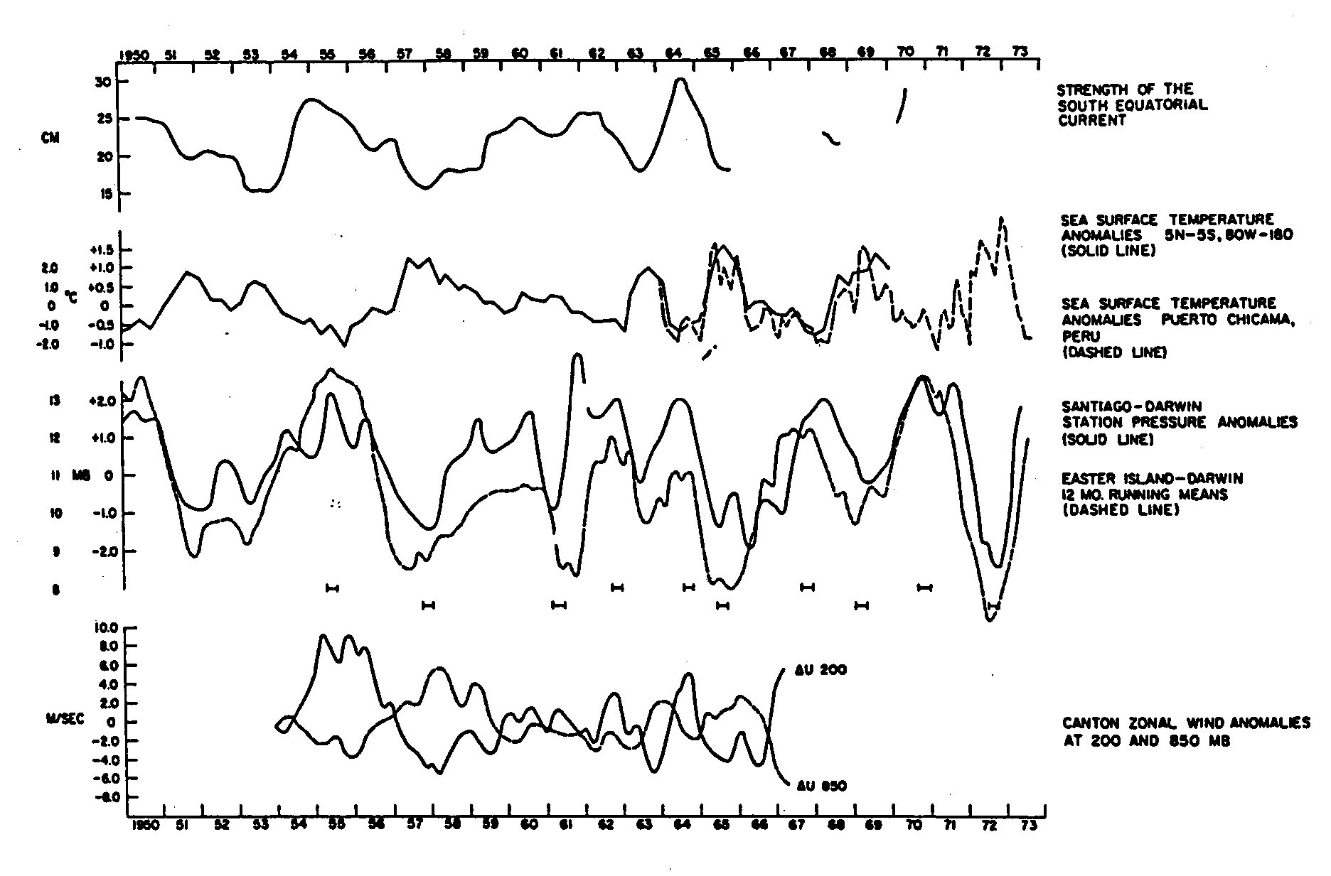
Figure 1.23 shows time-series of various oceanic and atmospheric variables at tropical stations during the period 1950 to 1973
taken from Julian and Chervin (1978). These data include the strength of the South Equatorial Current; the average SST over the
equatorial eastern Pacific; the Puerto Chicama (Peru) monthly SST anomalies; the 12 month running averages of the Easter Island-Darwin
differences in sea level pressure; and the smoothed Santiago-Darwin station pressure differences. The figure shows also the zonal wind
anomalies at Canton Island (3.S, 172.W) which was available for the period 1954-1967 only. The mutual correlation and particular phase
association of these time series is striking and indicate an atmosphere-ocean coupling with a time scale of years and a spatial scale
of tens of thousands of kilometres involving the tropics as well as parts of the subtropics. This coupled ocean-atmosphere phenomenon
is now referred to as ENSO, an acronym for El Niño-Southern Oscillation.
Figure 23. Composite low-pass filtered time series for various oceanographic and meteorological parameters involved
in the Southern Oscillation and Walker Circulation. Series are (top to bottom): the strength of the South Equatorial Current, a westward
flowing current just south of the equator; ocean surface temperature anomalies in the region 5oS to 5oN and
80oW to 180oW (solid line), and monthly anomalies of Puerto Chicama ocean surface temperature, dashed; two
Southern Oscillation indices, the dashed line being 12-month running means of the difference in station pressure Easter Island-Darwin and
the solid line being a similar quantity except Santiago is used instead of Easter Island; the bottom series are low-pass filtered zonal
wind anomalies (from monthly means) at Canton at 850 mb (dashed) and 200 mb (solid). The short horizontal marks appearing between two
panels denote the averagingintervals used in compositing variables in cold water and El Niño situations. (From Julian and Chervin, 1978).
During El Niño episodes, the equatorial waters in the eastern half of the Pacific are warmer than normal while SSTs west of the date
line are near or slightly below normal. Then the east-west temperature gradient is diminished and waters near the date line may be as
warm as those anywhere to the west (≈ 29oC). The region of heavy rainfall, normally over Indonesia, shifts eastwards so that Indonesia
and adjacent regions experience drought while the islands in the equatorial central Pacific experience month after month of torrential
rainfall. Near and to the west of the date line the usual easterly surface winds along the equator weaken or shift westerly (with
implication for ocean dynamics), while anomalously strong easterlies are observed at the cirrus cloud level. In essence, in the atmosphere
there is an eastward displacement of the Walker Circulation.
1.9 The Madden-Julian Oscillation, Westerly wind bursts
As well as fluctuations on an interannual basis, the Walker Circulation appears to undergo significant fluctuations on intraseasonal
time scales. This discovery dates back to pioneering studies by Madden and Julian (1971, 1972) who found a 40-50 day oscillation in
time series of sea-level pressure and rawinsonde data at tropical stations. They described the oscillation as consisting of
global-scale eastwardpropagating zonal circulation cells along the equator. The oscillation appears to be associated with intraseasonal
variations in tropical convective activity as evidenced in time series of rainfall and in analyses of anomalies in cloudiness and OLR.
The results of various studies to the mid-80s are summarized by Lau and Peng (1987). They list the key features of the intraseasonal
variability as follows:
i. There is a predominance of low-frequency oscillations in the broad range from 30-60 days;
ii. The oscillations have predominant zonal scales of wavenumbers 1 and 2 andpropagate eastward along the equator year-round.
iii. Strong convection is confined to the equatorial regions of the Indian Ocean and western Pacific sector, while the wind pattern
appears to propagate around the globe.
iv. There is a marked northward propagation of the disturbance over India and East Africa during summer monsoon season and, to a
lesser extent, southward penetration over northern Australia during the southern summer.
v. Coherent fluctuations between extratropical circulation anomalies and the tropical 40-50 day oscillation may exist, indicating
possible tropical-midlatitude interactions on the above time scale.
vi. The 40-50 day oscillation appears to be phase-locked to oscillations of 10-20 day periods over India and the western Pacific.
Both are closely related to monsoon onset and break conditions over the above regions.
Figure 24 shows a schematic depiction of the time and space variations of the circulation cells in a zonal plane associated with
the 40-50 day oscillation as envisaged by Madden and Julian (1972).
Figure 24. (a) Schematic depiction of the time and space variations of the disturbance associated with the 40-50 day
oscillation along the equator. The times of the cycles (days) are shown to the left of the panels. Clouds depict regions of enhanced
large-scale convection. The mean disturbance pressure is plotted at the bottom of each panel. The circulation on days 10-15 is quite
similar to the Walker circulation shown in Fig. 15. The relative tropopause height is indicated at the top of each panel. (b) shows
the mean annual SST distribution along the equator. The 40-50 day wave appears strongly convective when the SST is greater than
27oC as in panels 2-5 in (a). Panel (c) shows the variations of pressure difference between Darwin and Tahiti. The swing
is reminiscent of the SO, but with a time scale of tens of days rather than years. (From Webster, 1987b)
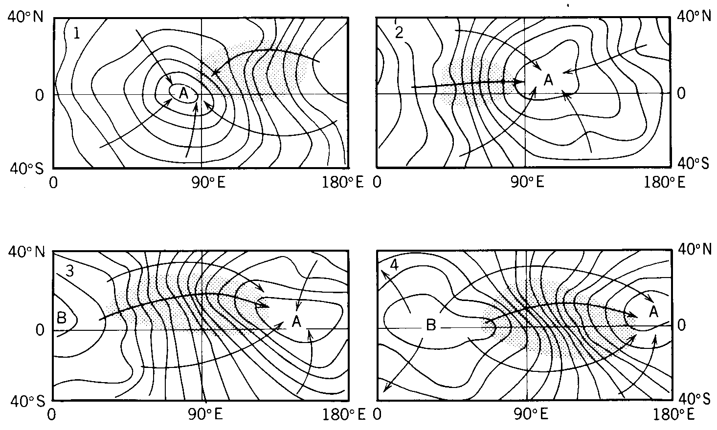
Figure 25 shows the eastward propagation of the 40-50 day wave in terms of its velocity potential in the Eastern Hemisphere.
The four panels, each separated by five days, show the distributions of the velocity potential at 850 mb. The centre of the ascending
(descending) region of the wave is denoted by A (B). As the wave moves eastwards, it intensifies as shown by the increased gradient.
Furthermore, and very important, as centre A moves eastwards from the southwest of India (which lies between 70.E and 90.E) to the east
of India, the direction of the divergent wind over India changes from easterly to westerly. Notice also that as centre A moves across
the Indian region that the gradient of velocity potential intensifies to the north as indicated by the movement of the stippled regions
in panels 2 and 3. Thus, depending on where the centres A and B are located relative to the monsoon flow, the strength of the monsoon
southwesterlies flowing towards the heated Asian continent will be strengthened or weakened. Thus we can the importance of the phase
of the MJO on the mean monsoonal flow.
Figure 25. (a) The latitude-longitude structure of the 40-50 day wave in the Eastern Hemisphere in terms of 850 mb
velocity potential. Units 10-6 s-1. The arrows denote the direction of the divergent part of the wind and the stippled region the
locations of maximum speed associated with the wave. Letters A and B depict the centres of velocity potential, which are seen to move
eastwards. Centre A may be thought of as a region of rising air and B a region of subsidence. (From Webster 1987b)
According to Lau and Peng, the most fundamental features of the oscillation are the perennial eastward propagation along the equator
and the slow time scale in the range 30-60 days. To date, observational knowledge of the phenomenon has outpaced theoretical
understanding, but it would appear that the equatorial wave modes to be discussed in Chapter 3 play an important role in the dynamics
of the oscillation.
Furthermore, because of the similar spatial and relative temporal evolution of atmospheric anomalies associated with the 40-50 day
oscillation and those with ENSO, it is likely that the two phenomena are closely related (see. e.g. Lau and Chan, 1986). Indeed, one
might view the atmospheric part of the ENSO cycle as fluctuations in a longer-term (e.g. seasonal average of the MJO). Two early
observational studies of the MJO are those of Knutson et al., (1986) and Knutson and Weickmann (1987). A review of early theoretical
studies is included in the paper by Blad┤e and Hartmann (1993) and a recent reviews of observational studies are contained in papers
by Madden and Julian (1994) and Yanai et al. (2000).
One might view the Walker Circulation as portrayed in Figs. 15 and 21 as an average of several cycles of the MJO.
Animations of satellite imagery during MJO events
Click here for an animation of infrared geostationary satellite centered
on the Equator over the Indian Ocean during an MJO event in 2011. (39 Mb)
Click here for an animation of infrared geostationary satellite centered
on the Equator over the Maritime Continent during an MJO event in 2011. (86 Mb)
1.10 Monsoons
The term monsoon originates from the Arabic "Mausim", a season, and was used to describe the change in the wind regimes as the
northeasterlies retreated to be replaced by the southwesterlies or vice versa. The term is be used here to describe the westerly air
stream (southwesterly in the NH, northwesterly in the SH) that results as the trade winds cross the equator and flow into the equatorial
trough. Accordingly, the term refers to the wind regime and not to areas of continuous rain etc., which are associated with the monsoon.
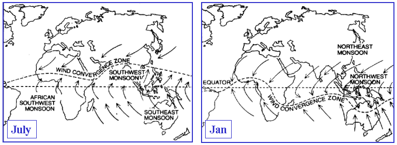
Figure 26 shows the typical low-level flow and other smaller scale features associated with the (NH) summer and winter monsoons in the
Asian regions.
Figure 26. Schematic of low-level air flow patterns near the Equator in January and July showing the main regions of
cross equatorial flow in the monsoon regions. (From ....)
Two main theories have been advanced to account for the monsoonal perturbations.
1.10.1 The regional theory
The regional theory regards the monsoon perturbations as low-level circulation changes resulting entirely from the large-scale heating
and cooling of the continents relative to oceanic regions. In essence the monsoon is considered as a continental scale "sea breeze"
where air diverges away from the cold winter continents and converges into the heat lows in the hot summer continents. The flow at higher
levels is assumed to play a minor role.
1.10.2 The planetary theory
With the great increase in upper air observations during the second half of this century, marked changes in the upper tropospheric flow
patterns have been found to accompany the onset of monsoonal conditions in the lower levels. In particular, marked changes in the
position of the subtropical jet stream accompany the advance of the monsoonal winds.
There are several objections to the regional theory. For example, monsoonal circulations are observed over the oceans, well removed
from any land mass, and the heat low over the continents is often remote from the main monsoonal trough. Moreover, the seasonal
displacement of surface and upper air features is well established from mean wind charts. This displacement is on a global scale, but
is greatest over the continental land masses, especially the extensive Asian continent. Hence an understanding of planetary circulation
changes in conjunction with major continental perturbations is necessary in understanding the details of the monsoonal flow.
Figure 27 shows Air flow patterns and primary synoptic- and smaller scale features that affect cloudiness and precipitation in the
summer and winter monsoon regions.
Figure 27. Air flow patterns and primary synoptic- and smaller scale features that affect cloudiness and precipitation
in the region of (a) the summer monsoon, and (b) the winter monsoon. In (a), locations of June to September rainfall exceeding 100 cm
the land west of 100oE associated with the southwest monsoon are indicated. Those over water areas and east of 100oE
are omitted. In (b) the area covered by the ship array during the winter MONEX experiment is indicated by an inverted triangle.
(From Houze, 1987)
1.10.3 Monsoon variability
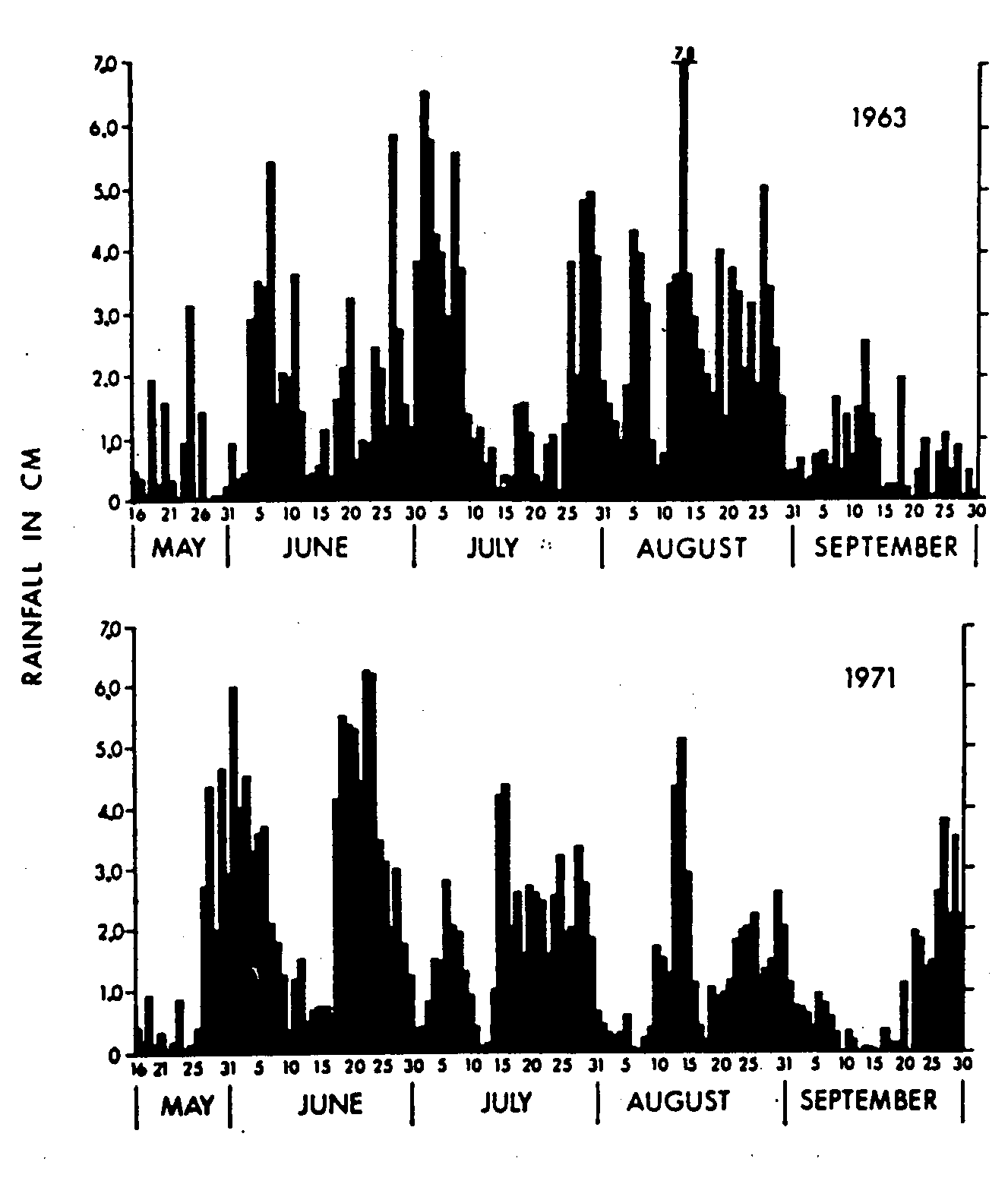
Superimposed upon the seasonal cycle are significant variations in the weather of the tropical regions. For example, in the monsoon
regions the established summer monsoon undergoes substantial variations, vacillating between extremely active periods and distinct "lulls"
in precipitation. The latter are referred to as "monsoon breaks". An example of this form of variability is shown in Fig. 28 which
summarizes the monsoon rains of two years, 1963 and 1971, along the west coast of India. The "active periods" are associated with groups
of disturbances and the "breaks" with an absence of them,. Usually, during the break, precipitation occurs far to the south of India and
also to the north along the foothills of the Himalaya. Such variability as this appears characteristic of the precipitating regions of
the summer and winter phases of the Asian monsoon and the African monsoon.
Figure 28. Daily rainfall (cm/day) along the western coast of India incorporating the districts of Kunkan,
Coastal Mysore and Kerala for the summers of 1963 and 1971. (From Webster, 1983)
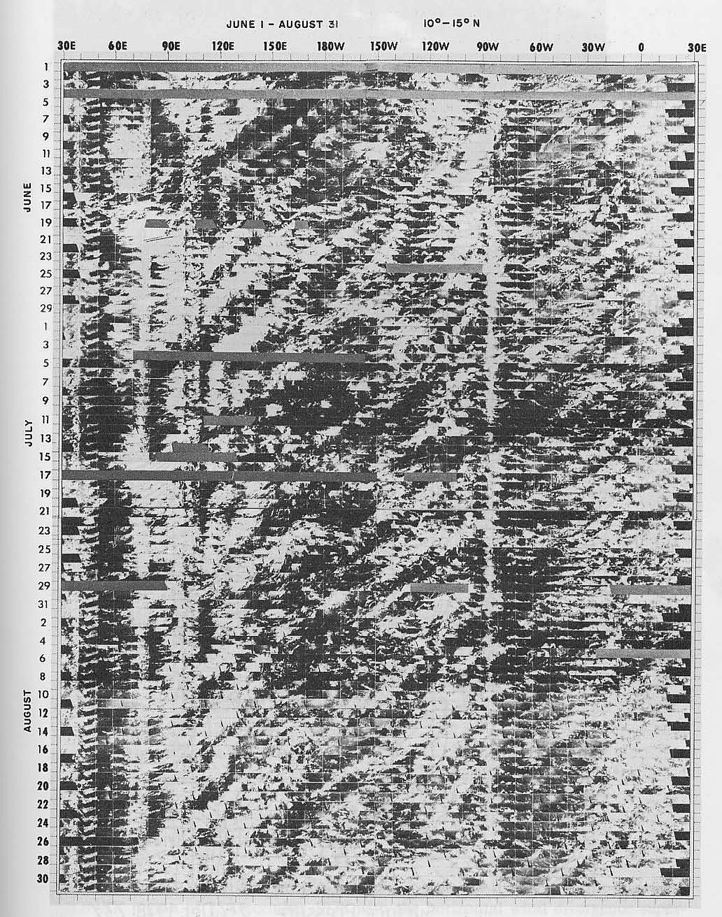
The individual disturbances of the active monsoon and those associated with the near- equatorial troughs move westward in a fairly
uniform manner. Such movement is shown clearly in Fig. 29. The westward movement is apparent in the bands of cloudiness extending
diagonally from right to left across the time-longitude sections.
Figure 29. Time-longitude section of visible satellite imagery for the latitude band 10-15.N of the tropics. Cloud
streaks moving from right to left with increasing time denotes westward propagation. Note that there is typically easterly flow at
these latitudes. (From Wallace, 1970)
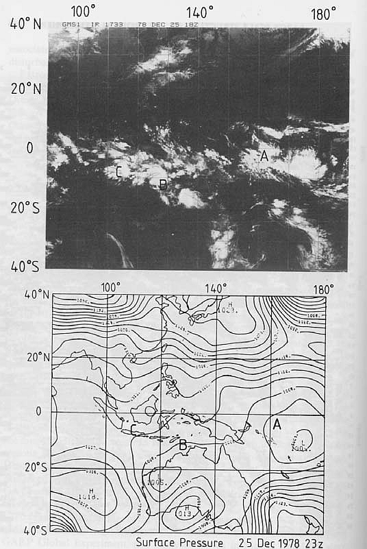
To illustrate the structure of propagating disturbances, Webster (1983) discusses a particular example taken from Winter-MONEX) in
1978. Figure 30 shows the Japanese geostationary satellite (GMS) infra-red (IR) satellite picture at 1800 UTC on 25 December 1978 for
the Winter-MONEX region with the .2300 UTC surface pressure analysis underneath. Figure 31 shows the corresponding wind fields at
250 mb and 950 mb. What is striking is the existence of significant structures in the satellite cloud field which have no obvious
signature in the surface pressure field. Indeed, the tropical portion of the pressure field is relatively featureless, except for
the heat low in north-western Australia and the broad trough that spans the near equatorial region of the southern hemisphere just west
of the date line. The most that one can say is that the major cloud regions appear to reside about the axis of a broad equatorial trough.
Figure 30. The winter MONEX region of 25 December 1978. Upper left panel shows the GMS IR satellite picture with the
surface-pressure pattern shown on lower panel. Both panels are on the same projection. Pressure analysis after McAvaney et al. (1981):
Letters A. B and C identify synoptic-scale disturbances referred to in the text. The 250 mb (upper right panel) and 950 mb (lower right
panel) wind fields for the same times with the horizontal wind divergence superimposed in the 20oS-20oN latitude
strip. In the upper troposphere areas the divergence are stippled whereas in the lower troposphere areas of convergence are stippled.
Stippled areas denote divergence magnitudes greater than 5 × 10⁻⁴ s-11.(From Webster, 1983)
Webster considers three major regions of deep high cloudiness denoted by A, B and C which appear to be synoptic scale disturbances.
He shows that these can be associated with areas of low-level convergence in the 950 mb wind field lying beneath areas of upper-level
divergence at 200 mb. The implication is that these are each deep divergent systems. Such properties: lower tropospheric convergence,
deep penetrative convection and upper-level divergence appear characteristic of the synoptic-scale tropical disturbances of the ITCZ
and the major convective zones of the monsoon.
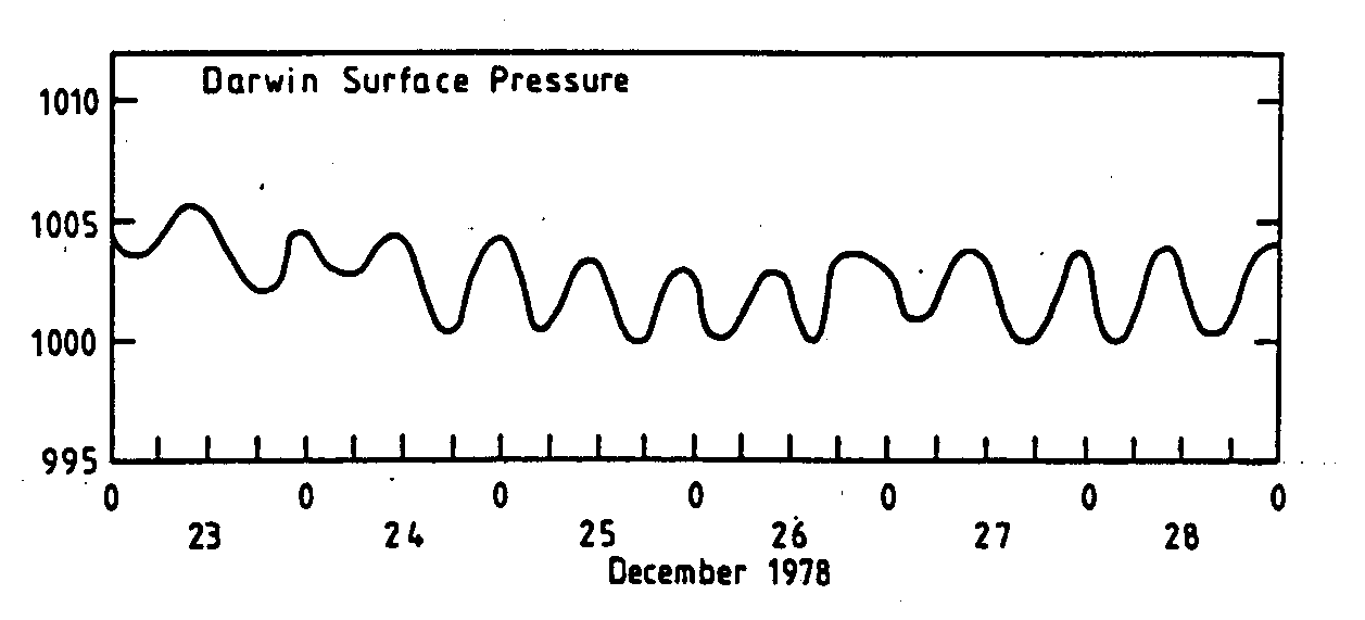
Figure 31 shows the surface pressure trace for Darwin from 23 - 28 December 1978, covering the period of the case study presented
in Figs. 30. The major variation in the pressure is associated with the semi-diurnal oscillation which has an amplitude of about 4 mb.
Little alteration to the semi-diurnal trend is apparent near 25 December 1978 which coincides with the existence there of the disturbance.
Indeed at low latitudes only on rare occasions with the passage of a tropical cyclone will the synoptic-scale pressure perturbations be
larger than the semi-diurnal variation.
Figure 31. The variation of surface pressure at Darwin for the period 23 - 28 December 1978. The structure is dominated
by the semi-diurnal atmospheric tide. From ...
1.12 Moist convection and convective systems
A major feature of tropical weather systems is the occurrence of deep convective cloud systems. Here we review of basic concepts
necessary to understand moist convection. We begin here with a brief discussion of convective instability and go on to examine three
types of convection: shallow convection, which as the name suggests has a limited vertical extent, and deep convection, which extends
through much or all of the troposphere and intermediate convection, where the cloud tops remain below the freezing level, which is
about 5.5 km high in the tropics.
1.12.1 Convective instability
The occurrence of moist convection in the atmosphere is frequently explained in terms the behaviour of an ascending air parcel that
does not mix with its environment. When an unsaturated air parcel is lifted adiabatically, it expands and and cools. Since the maximum
amount of water vapour it can hold decreases strongly as its temperature decreases, it eventually reaches a level at which it becomes
saturated. This is the so-called lifting condensation level, or LCL. If the parcel is lifted above this level, water progressively
condenses and the latent heat that is released reduces the rate at which the parcel cools. Typically a parcel is still denser than its
environment at the LCL and is therefore negatively buoyant. However, if the lifting continues, it may reach a level at which it becomes
lighter than its environment and therefore positively buoyant. This level is called the level of free convection (LFC). Above this level
the parcel can accelerate under its own buoyancy force until at some further level it again becomes neutrally buoyant. This level is
called the level of neutral buoyancy, or LNB. Above the LNB the parcel has negative buoyancy and usually rapidly decelerates.
1.12.2 Aerological diagrams
The various levels described above are usually estimated on the basis of an aerological diagram, which is a judiciously transformed
thermodynamic diagram. In its most basic form, a thermodynamic diagram is one in which the pressure p and specific volume α are
plotted on the ordinate and abscissa, respectively. Then according to the equation of state (pα = RT, where p is the pressure,
α is the specific volume, R is the specific gas constant and T is the temperature), the isotherms are rectanglar hyperbolae.
The state of a parcel of dry air can be represented by a point in such a diagram and the change in state as the pressure and specific
volume change can be represented as a curve. For example, an isothermal change is represented by a rectangular hyperbola. The
p-α-diagram is of limited practical use in meteorology because the specific volume is not a quantity that is measured.
An aerological diagram is transformed version in which more relevant meteorological variables are displayed and lines representing
state changes associated with important atmospheric processes are plotted. There are various kinds of such diagrams, one being the
tephigram and another the skew-T log-p diagram. In the latter diagram the isobars are straight horizontal lines and are plotted with a
logarithmic scale with pressure decreasing upwards so that the ordinate is approximately equal to height. The isotherms are straigt lines
that run upwards to the right at an angle of 45 degrees. Also plotted are the dri-adiabats, curves curves on which the potential
temperature is constant; the moist adiabats, curves on which the pseudo-equivalent potential temperature is constant; and curves of
constant saturation mixing ratio. While the state of a sample of dry air is represented by a single point in the diagram, that of a moist
sample requires two points, one corresponding to the pressure and temperature of the parcel and the second corresponding to the pressure
and dew-point temperature, Td. The saturation mixing ratio line that intersects the point (p,Td) gives the water
vapour mixing ratio of the parcel. The state of the atmosphere at a given location and time obtained from a radiosonde sounding can be
plotted as pair of curves (p,T) and (p,Td).
Figure 32 shows a skew-T log-p diagram with a mean tropical sounding for the Atlantic hurricane season plotted. The skew-T log-p
diagram can be used to investigate changes of state of an air parcel as its pressure changes.
Figure 32: A skew-T log-p aerological diagram with a mean sounding for the Atlantic Hurricane season plotted. The red
curve is the temperature and the blue curve the dew-point temperature. From ...
1.12.3 CAPE and CIN
The amount of energy that a particular parcel could achieve by rising from a particular level zi to its LNB is called the convective available potential energy (CAPE) and may be written as
where b is the generalized buoyancy force per unit mass that acts on on the parcel and dl is a unit
vector along the path of the displacement. If the parcel rises vertically, this integral may be written
where z measures height (normal to geopotential surfaces) and b is the vertical component of the buoyancy force. Using the equation of
state in the form p = ρRTρ where Tρ is the density temperature, and assuming that the environment is in
hydrostatic equilibrium, we can show that
It follows that CAPEi is proportional to the area enclosed by the density temperature of the lifted parcel and that of the
environment, respectively, on a thermodynamic diagram whose coordinates are linear in temperature and in log p. CAPE depends on the initial
parcel, i, and on the thermodynamic process assumed in lifting the parcel. It is defined only for those parcels that are positively
buoyant somewhere on the sounding.
The amount of work that must be expended to lift a parcel to its level of free convection is called the convective inhibition (CIN)
and is given by the integral
Again, if the parcel is lifted vertically, this integral may be written
The negative area represents, in essence, a potential barrier, or potential well, to convection, that prevents it from occurring
spontaneously. There is no analogy to this potential barrier in dry convection; this is one distinguishing feature between moist and dry
convection, although not only one. The existence of a potential barrier allows CAPE to accumulate under certain meteorological conditions,
creating the possibility that it may be released explosively at a later time.
1.12.4 Types of convection
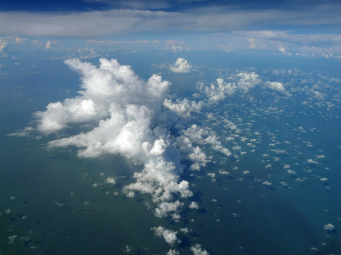
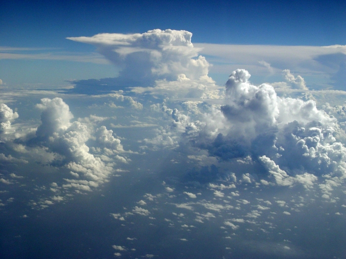
Figure 33 shows some photographs of tropical convection in a variety of forms. It is sometimes useful to divided convection into
three types, shallow convection, intermediate convection and deep convection as follows.
Shallow convection
Shallow convection refers to convective clouds that have a limited vertical extent, with tops perhaps no more than one or two
kilometres. Generally such clouds do not precipitate. They are often referred to as "trade-wind cumuli". Theoretical treatments of shallow
convection assume that the clouds do not produce precipitation. Fields of shallow convection are important for the larger scale because
the convection facilitates mixing, leading to a vertical transport of heat and moisture into the cloud layer and the transport of dry air
through intra-cloud subsidence into the subcloud layer. In this way, shallow convection counteracts the drying and warming effects of
large-scale subsidence regions. Examples of shallow convection can be seen in all the panels Fig. 33 suggesting that such convection is
ubiquitous in the tropics.
(a)
(b)
(c)
(d)
(e)
(f)
(g)
(h)
Figure 33: Some photographs of tropical convection convection. See text for discussion.
Click here for a time-lapse movie of shallow convection in the tropics. (161 Mb)
Intermediate convection
Intermediate convection refers to convective clouds that produce heavy showers, but which do not extend far enough in the vertical to
contain ice. In the tropics the freezing level is around 5.5 km. In these clouds the processes leading to the rain do not involve ice
processes. Thus rain drops are produced only by the collision and coalescence of smaller drops. We refer to the rain produced in such
clouds as warm-rain. Examples include so called cumulus congestus clouds, examples of which are shown in Fig. 33 (a), (c) and
(e).
Click here for a time-lapse movie of a tropical rain shower. (3.3 Mb)
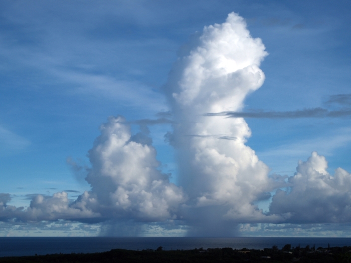
Deep convection
Deep convection refers to precipitating clouds that extend vertically through a significant depth of the troposphere, typically well
bove the freezing level. Besides producing heavy local precipitation, they may give rise to thunder and lightning. An important
characteristic of precipitating convection is the production of strong downdraughts when precipitation evaporates in subsaturated air, or
when it melts at the freezing level. An example is shown in the distance in Fig. 34(c). Deep convective clouds usually produce extensive
anvils of ice particles that often outlive the convective cells that generate them. These anvil clouds take on a dynamics of themselves
with slow ascent above the freezing level and subsidence below generated by moderate to weak precipitation below them. There may be
significant convergence near the freezing level induced by the sharp increase in the fall speed of hydrometeors as snow melts to form
raindrops.
The downdraughts that accompany deep convective systems can have an important stabilizing effect on the subcloud air, making it cooler
and drier. However, once a convective cell has developed, lifting of air ahead along the boundaries of the low-level cold outflow can
trigger new convection. In this manner, convective systems have a propensity to generate new cells that subsequently aggregate.
Over the ocean, surface fluxes of heat and moisture lead to a warming and moistening of the downdraught air on time scales on the
order of half a day, thereby restoring convective instability.
The warming of the atmosphere in regions of convection is a result not only of the direct release of latent heat in clouds, but also
by the subsidence in the environment of clouds brought about by horizontally-propagating gravity waves. In this way, a whole region
including clouds and their environments can undergo warming.
Typical updraughts speeds in deep convection over the oceanic are typically only a few m s-1, somewhat weaker than typical
speeds in deep convection over land in the middle latitudes, where updraught smay reach 15 m s-1, or more
(see Lucas et al. 1994 ). However, tropical clouds are generally deeper than their middle latitude
counterparts as the tropopause is several kilometres higher in the tropics. An interesting paper on this topic is that by
Zipser (2003) .
Time-lapse videos of tropical thunderstorms
Click here
for a time-lapse movie of a tropical thunderstorm: looking north from Darwin, Australia (350 Mb)
1.12.5 Understanding the effects of deep convection in tropical weather systems
An important consideration in understanding the interaction between deep convection and the broadscale flow in tropical disturbances is to realize that deep convection occurs as a result of
convective instability. First, some air parcels must be brought to their LFC, either as a result of boundary layer turbulence or as a result of mechanical lifting at the spreading outflow boundary
produced by previous convection. Above the LFC, air parcels can rise through the depth of the troposphere in favourable conditions and they may even overshoot their LNB into the lower stratosphere.
It turns out that usually, only air parcels below a few 100 m to 1 km have any CAPE so that only these can rise through a deep layer. Thus deep convection typically peels of a layer of warm moist air
near the surface and expels (or detrains) it into the upper troposphere near the level of neutral buoyancy. At air parcels rise they entrain air from their environment. The entrained air is generally
unsaturated and slightly cooler than the air parcel so that entrainment tends to reduce the amount of buoyancy in the updraught below that which would be predicted by an aerological diagram and
tends to lower the LNB.
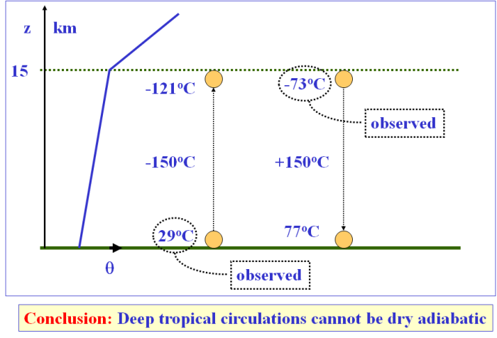
When an air parcel ascends in a stably stratified environment, it expands and cools. As long as it remains unsaturated it cools at the dry adiabatic lapse rate (10oC km-1) and if a parcel could
be lifted dry adiabatically from the surface in the tropics (say with a temperature of 29oC) to the tropopause (say at a height of 15 km), it would have a temperature when it reached the tropopause
of -121oC (see Figure 5.3). Since temperatures near the tropical tropopause are typically around -73oC, the air parcel would have a huge negative buoyancy when it got there and the
lifting would require a huge amount of work to be done to lift the parcel. Since there is no conceivable mechanism in the atmosphere that could supply the needed work, we must conclude that the air parcel must
rise in cloud, where the cooling can be offset by latent heat release, first as condensation occurs and later as freezing occurs.
Figure 34: Implications of a dry adiabatic circulation. An air parcel rising dry adiabatically from the surface at a typical
temperature of 29 C would arrive at the tropopause, assumed to be 15 km high, at a temperature of -121oC, compared with a
typical observed value of -73oC. Conversely, an air parcel subsiding dry adiabatically from the tropical tropopause at a
typical temperature of -73oC would arrive at the surface with a temperature of 77oC. In both cases, a large amount
of work would be required to offset the opposing buoyancy force.
A similar argument can be used to argue that an air parcel cannot descend from the tropopause level to the surface unless it cools
to offset the 150oC temperature rise that would be produced as a result of adiabatic compression. Typically, the subsiding air
parcel with an initial temperature at the tropopause of -73oC would have to cool radiatively, the normal rate being on the
order of 2oC per day. Thus, in order to arrive at the surface with a temperature of 29oC, the parcel would have to
cool by 48oC, which could be accomplished only after 24 days. Since an air parcel can rise from the surface to the tropical
tropopause in about 20 minutes, mass conservation would require that the area of descent be much larger than the area of ascent. This
result would explain why the areas of active convection in Fig. 3 occupy a rather small fractional area in the tropics (remember that
the areas of convective updraughts are much smaller in area than the cirrus cloud they give rise to).
1.12.6 Further reading on convection
Jakob, C., 2001: Cloud parametrization - Progress, Problems and Prospects. ECMWF Seminar.
(click here) This paper is an erudite review of some of the issues involved in representing
sub-grid-scale clouds in models.
Betts, A. K., and C. Jakob. 2002a: Evaluation of the diurnal cycle of precipitation, surface thermodynamics, and surface fluxes
in the ECMWF model using LBA data. J. Geophys. Res., 107, (click here)
Betts, A. K., and C. Jakob. 2002b: Evaluation of the diurnal cycle of precipitation, surface thermodynamics, and surface fluxes
in the ECMWF model using LBA data. J. Geophys. Res., 107, (click here)
Click here for a review of
atmospheric moist convection by B. Stevens.
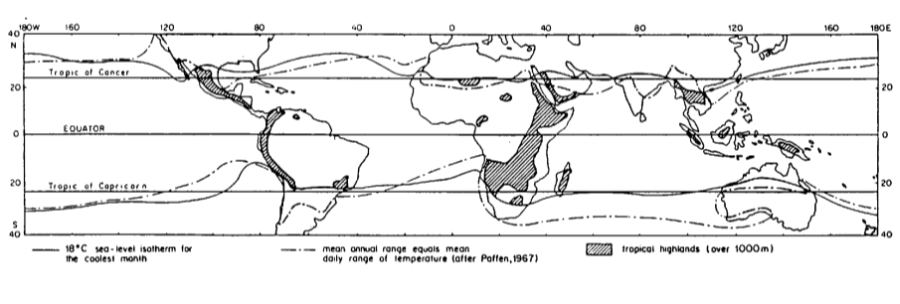
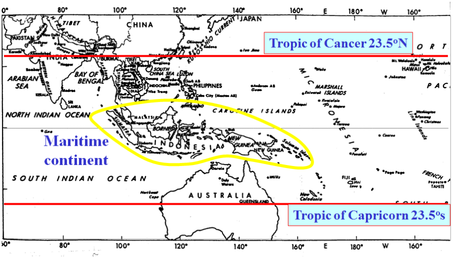

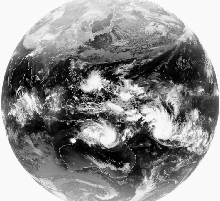

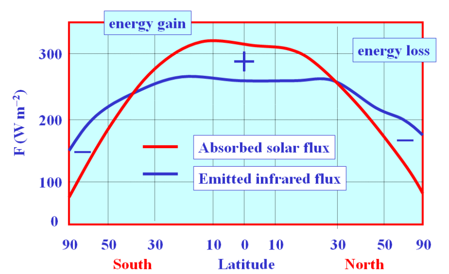

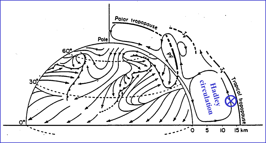
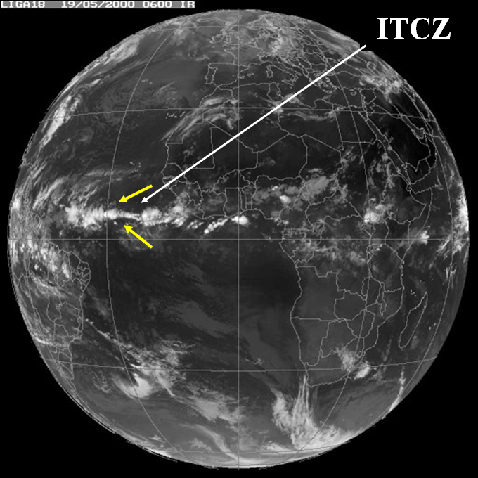

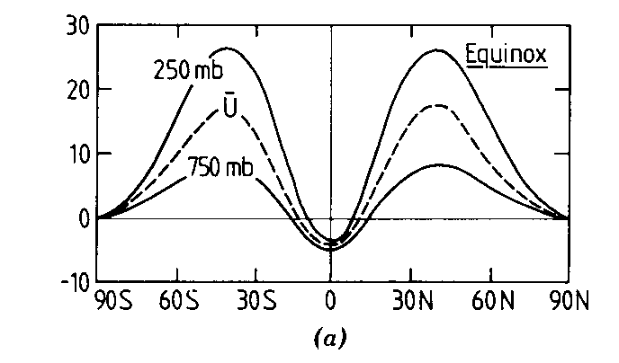
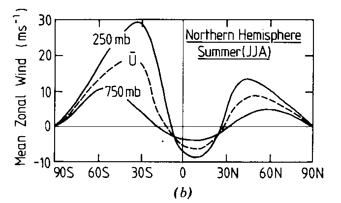
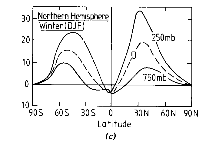
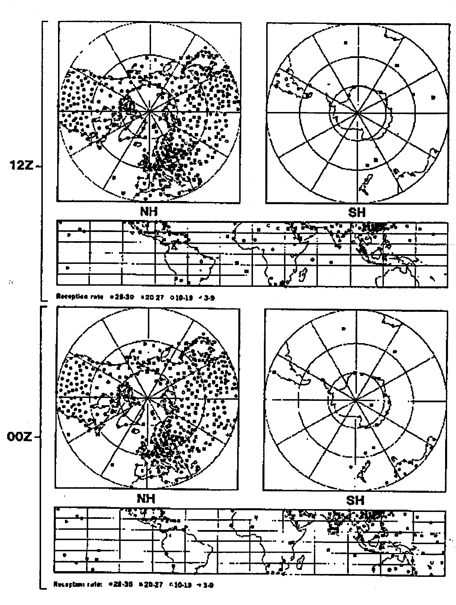

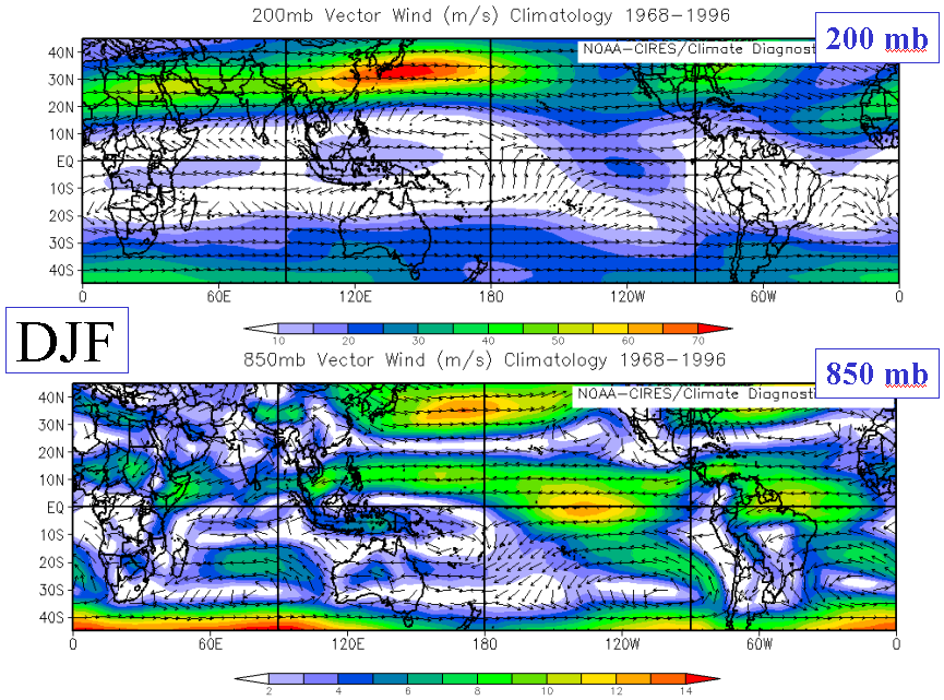
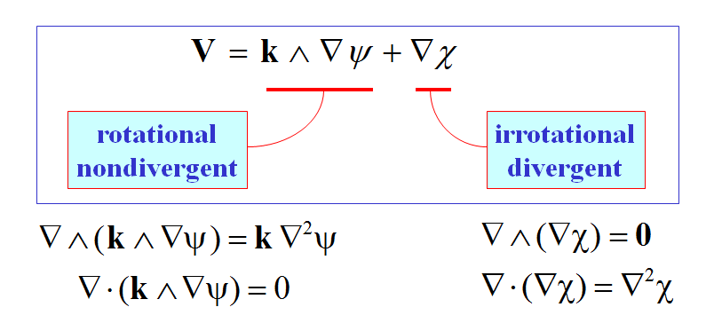


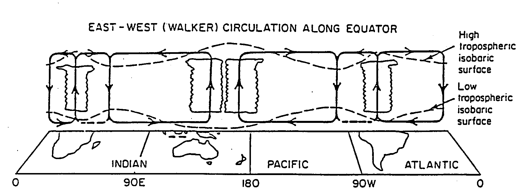

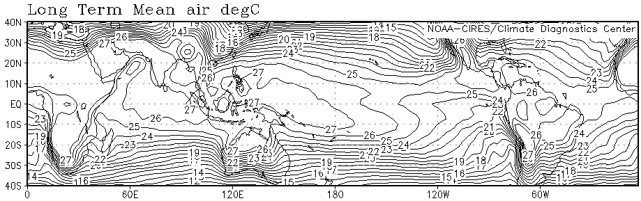
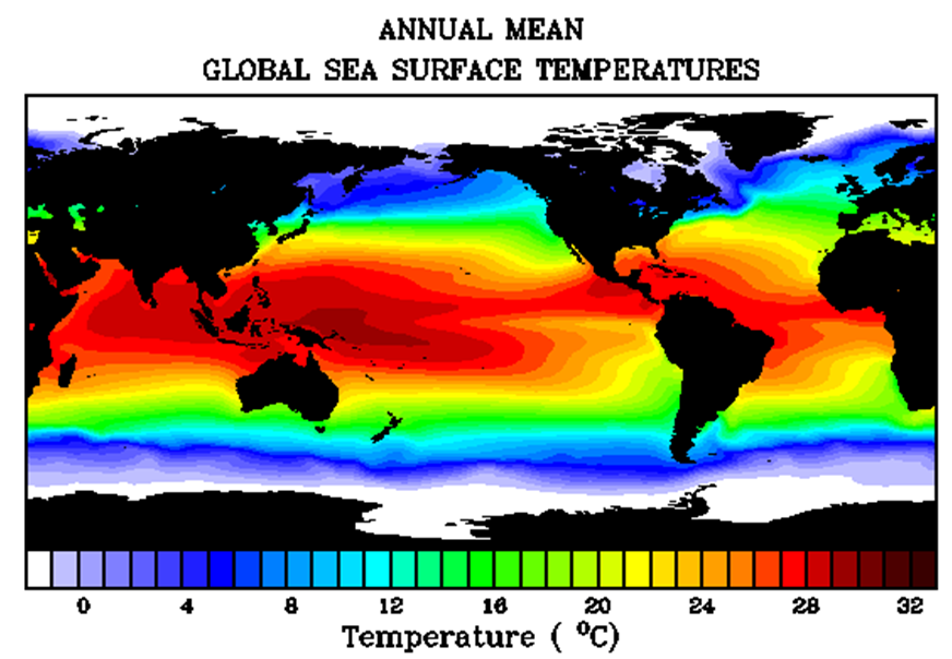
 Figure missing

 (a)
(a)
 (b)
(b)
 (a)
(a)
 (b)
(b)


 (b)
(b)
 (d)
(d)
 (f)
(f)
 (h)
(h)